Quantum Phase Transitions

A quantum phase transition is a qualitative change in the ground-state phase of a many-body system at zero temperature as a nonthermal parameter in its Hamiltonian is varied. For a family

$$H(g),$$

the control parameter $g$ may represent a magnetic field, pressure-dependent coupling, interaction-to-hopping ratio, density, or another quantity that changes the competition among terms in $H$.

The sharp transition is a bulk statement. If $E_0(g,L)$ is the ground-state energy of a system with linear size $L$, then the ground-state energy density is

$$e_0(g) = \lim_{L\to\infty} \frac{E_0(g,L)}{L^d}.$$

A transition occurs at $g=g_c$ when the thermodynamic-limit ground state cannot be continued through $g_c$ without a nonanalytic change in an appropriate bulk observable, response, correlation structure, excitation spectrum, or phase invariant.

Quantum fluctuations drive the transition because competing terms in $H(g)$ generally do not commute. Temperature is set to zero in the definition, but a zero-temperature critical point can organize a broad finite-temperature crossover regime. A finite-temperature crossover is not itself the quantum phase transition.

Canonical Scope

This page is the canonical home for the general many-body concept of a quantum phase transition. It owns:

• parameter-driven changes of ground-state phase at $T=0$;
• finite-size versus thermodynamic-limit singularities;
• first-order and continuous quantum transitions;
• gap closing, correlation-length scaling, and the dynamical exponent;
• the finite-temperature quantum-critical regime;
• imaginary-time and quantum-to-classical scaling intuition;
• finite-size diagnostics and failure modes;
• the transverse-field Ising chain and Bose–Hubbard transition as benchmarks.

Focused pages retain neighboring ownership:

• Phases of Matter in Many-Body QM owns the general definition, robustness criteria, and diagnostic fingerprint for phases; this page owns the zero-temperature boundaries between them.
• Thermodynamic Limit owns the general construction of bulk limits and the broad finite-size-scaling preview.
• Critical Exponents and Scaling owns the exponent dictionary, scaling identities, correction terms, dynamic scaling, and covariance-aware finite-size collapse; the Critical Exponent Glossary gives the compact thermal-to-quantum dictionary.
• Spontaneous Symmetry Breaking Preview owns source-selected broken-symmetry states and noncommuting source and volume limits.
• Ising Chain owns its compact reference definition. Bose–Hubbard Model owns the full lattice-boson conventions and model-specific mean-field boundary; its model card remains the compact lookup entry.
• Universality owns universality-class criteria, universal versus nonuniversal data, and the limits of quantum-to-classical class matching. Renormalization Group Preview owns fixed points and coupling-space flow. Landau Theory owns uniform order-parameter potentials; Topological Order Preview owns the first treatment of phase diagnostics beyond local symmetry breaking.
• Entanglement Entropy owns the finite-system entropy definition; this page only uses entanglement as one diagnostic of critical structure.
• Entanglement Entropy in Many-Body Systems owns spatial scaling laws and the one-dimensional conformal formulas.
• Area Laws owns the precise gapped-chain theorem, higher-dimensional open status, and boundary-normalized tests.
• Many-Body Entanglement Overview owns the broader audit of partition choice, state class, measure selection, and asymptotic evidence.

What Counts as a Phase Change?

Two parameter intervals represent distinct phases when no admissible smooth deformation connects their bulk ground states while preserving the properties used to define the phase. The relevant obstruction may involve:

• spontaneous breaking of a symmetry;
• a closing of the bulk excitation gap;
• a change in long-distance correlation behavior;
• a change in stiffness, compressibility, or quantized response;
• topological order or a symmetry-protected invariant;
• a change from a gapped phase to a stable gapless phase.

No single item is universal. A local order parameter works for many symmetry-breaking transitions but not for every topological transition. A gap can close along an entire phase rather than only at one point. First-order transitions can be controlled by competing ground states rather than a diverging correlation length.

The phase definition must therefore state:

1. the Hamiltonian family and control parameter;
2. the thermodynamic sequence and boundary conditions;
3. the symmetries or constraints held fixed;
4. the bulk observables or invariants used to distinguish phases;
5. the order of zero-temperature, source, and volume limits.

Why Finite Systems Usually Look Smooth

Suppose $H(g)$ depends analytically on $g$ and has an isolated, nondegenerate ground state in a finite-dimensional Hilbert space. In a neighborhood where the gap remains open, standard spectral perturbation theory makes the ground-state energy and projector analytic functions of $g$.

Consequently, a generic finite system exhibits a crossover rather than a sharp continuous transition. Levels with the same exact quantum numbers usually avoid crossing. An exact finite-size crossing can occur when symmetry places the states in different sectors or when additional integrability prevents hybridization, but an isolated crossing alone does not establish a bulk phase transition.

Define the finite-size spectral gap

$$\Delta_L(g) = E_1(g,L)-E_0(g,L).$$

Near a continuous quantum critical point, the minimum gap decreases as $L$ grows and vanishes only in the thermodynamic limit. Near a first-order transition, competing macroscopic states can instead produce an exponentially small avoided-crossing gap. The size dependence, symmetry sector, and identity of the excitation matter as much as the numerical value of $\Delta_L$.

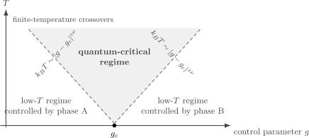
Schematic organization near a continuous quantum critical point. The sharp transition is the point $g_c$ at $T=0$. The dashed curves represent crossover scales $k_B T\sim|g-g_c|^{z\nu}$, not universal phase boundaries. Actual finite-temperature transitions, disorder, additional relevant couplings, or first-order behavior can alter this diagram.

First-Order and Continuous Transitions

The distinction is made from bulk singularities, not from whether a finite numerical curve looks steep.

First-order quantum transitions

Let

$$H(g) = H_0+gV.$$

For a nondegenerate finite-system ground state, the Hellmann–Feynman theorem gives

$$\frac{\partial E_0}{\partial g} = \langle V\rangle_0.$$

After division by volume and passage to the bulk limit,

$$\frac{d e_0}{dg} = \lim_{L\to\infty} \frac{\langle V\rangle_0}{L^d},$$

where the derivative exists. A discontinuity in this quantity signals a first-order transition. Physically, two macroscopically distinct ground states exchange stability.

At a first-order quantum transition:

• the order parameter or another first derivative can jump;
• the correlation length need not diverge;
• a finite system can show an exact or avoided level crossing;
• the minimum gap can be exponentially small in volume;
• hysteresis in a protocol may occur but is not the equilibrium definition.

Continuous quantum transitions

At a conventional continuous transition, the ground-state energy remains differentiable to lower orders while long-distance scales become singular. A correlation length commonly diverges as

$$\xi = a |\delta|^{-\nu}, \qquad \delta = \frac{g-g_c}{g_0},$$

where $a$ and $g_0$ are microscopic scales and $\nu$ is the correlation-length exponent.

The characteristic low-energy scale vanishes as

$$\Delta \sim E_0 |\delta|^{z\nu},$$

and the corresponding correlation time diverges:

$$\tau_\xi \sim \frac{\hbar}{\Delta} \sim \xi^z.$$

The exponent $z$ is the dynamical critical exponent. It states how time and space rescale near criticality:

$$\mathbf x \longrightarrow b\mathbf x, \qquad t \longrightarrow b^z t.$$

Power laws are common but not universal. Berezinskii–Kosterlitz–Thouless transitions have an essential rather than algebraic divergence of $\xi$. Infinite-randomness critical points can have activated rather than power-law dynamical scaling. A scaling form must be justified for the universality class under study.

Gap Closing: Important but Not a Standalone Definition

For a conventional continuous transition between two gapped phases, the bulk gap closes at $g_c$. This produces long correlation times and makes low-energy states sensitive to large distances.

Three qualifications are essential.

First, define which gap is being measured. In a symmetry-broken phase, the splitting between finite-size symmetry partners can vanish exponentially throughout the ordered phase, while the gap to a local bulk excitation remains nonzero away from criticality.

Second, a gapless phase can occupy a finite interval of $g$. The transition into that phase is not identified merely by observing one small gap.

Third, first-order transitions and level crossings can close a ground-state gap without producing scale-invariant fluctuations. Gap closing must be interpreted together with correlations, matrix elements, symmetry sectors, and size scaling.

Scaling Near a Continuous Critical Point

Near a scale-invariant critical point, an observable’s singular part can often be organized by a homogeneity relation. Measuring lengths in microscopic units, write

$$\begin{aligned} O_s(\delta,T,L,\{u_i\}) ={}& b^{-x_O} \mathcal F_O\!\left( \delta b^{1/\nu}, \frac{k_B T}{E_0}b^z, \frac{L}{b}, \{u_i b^{y_i}\} \right). \end{aligned}$$

Here:

• $x_O$ is the scaling dimension associated with $O$;
• $u_i$ are additional scaling fields;
• $y_i>0$ denotes a relevant perturbation;
• $y_i<0$ denotes an irrelevant perturbation;
• $y_i=0$ requires a separate marginal-flow analysis.

At $T=0$ and infinite volume, choosing

$$b = |\delta|^{-\nu}$$

reduces the long-distance behavior to powers of $|\delta|$ multiplied by scaling functions. For an order parameter $m$ on the ordered side,

$$m \sim (-\delta)^{\beta_{mathrm{op}}},$$

where $\beta_{mathrm{op}}$ is a critical exponent, not the inverse temperature.

When hyperscaling is valid, the singular ground-state energy density obeys

$$e_s \sim \xi^{-(d+z)}.$$

This relation can fail above an upper critical dimension or in the presence of dangerously irrelevant variables. Critical-exponent identities should not be applied without checking those assumptions.

Quantum Criticality at Nonzero Temperature

Temperature introduces a thermal time scale

$$\tau_T \sim \frac{\hbar}{k_B T}.$$

Away from $g_c$, the ground-state phase controls low-temperature behavior when

$$k_B T \ll \Delta(g).$$

Near criticality, the thermal scale exceeds the detuning gap when

$$k_B T \gtrsim \Delta(g).$$

Using $\Delta\sim|\delta|^{z\nu}$ gives the crossover scale

$$k_B T_\times \sim E_0 |\delta|^{z\nu}.$$

The region $T\gtrsim T_\times$ is often called quantum critical because neither adjacent zero-temperature phase supplies the only relevant low-energy description. Observables can show scaling governed by the nearby quantum critical fixed point.

This does not mean the system is in its ground state at finite temperature. Its equilibrium state is a thermal density operator, and the imaginary-time extent is finite. Nor is every line drawn around a quantum-critical fan a phase boundary. Many are crossovers, and a system may also contain genuine finite-temperature transition lines. Their thermodynamic definition, order, critical temperature, and finite-size diagnostics belong to Finite-Temperature Phase Transitions.

Imaginary Time and Effective Dimension

The equilibrium partition function is

$$Z = \operatorname{Tr} e^{-\beta H}, \qquad \beta = \frac{1}{k_B T}.$$

In an imaginary-time path integral, fields live on

$$0 \le \tau \lt \beta\hbar.$$

At $T=0$, the interval becomes infinitely long. A $d$-dimensional quantum system can therefore be represented by a classical statistical system with $d$ spatial coordinates plus one imaginary-time coordinate.

The phrase “effective dimension $d+z$” is a scaling statement, not generally a literal count of coordinates. Under critical rescaling,

$$d^d x\,d\tau \longrightarrow b^{d+z} d^d x\,d\tau.$$

When $z=1$ and the long-distance action can be made isotropic, the mapping resembles a classical model in $d+1$ Euclidean dimensions. For $z\ne1$, space and imaginary time scale anisotropically even though there is still only one time coordinate.

The transverse-field Ising model provides a precise benchmark: a $d$-dimensional quantum Ising model maps through a Trotter construction to an anisotropic classical Ising model in $d+1$ dimensions. More general quantum-to-classical mappings can be modified by Berry phases, fermionic signs, long-range temporal interactions, dissipation, quenched disorder, constraints, or topological terms. “Add one dimension” is useful intuition, not a universal theorem about all quantum critical points.

Benchmark I: Transverse-Field Ising Chain

The Transverse-Field Ising Model dossier owns the compact model record, limiting cases, and validation contracts. The teaching article owns duality, the exact-solution development, parity sectors, and model-specific entanglement. Here the chain serves a narrower purpose: it makes the general scaling concepts concrete.

Consider

$$H = -J \sum_{j=1}^{L} \sigma_j^z\sigma_{j+1}^z - gJ \sum_{j=1}^{L} \sigma_j^x, \qquad J>0.$$

The dimensionless field $g$ competes with the Ising exchange. The Hamiltonian has a global $\mathbb Z_2$ symmetry generated by

$$\mathcal P = \prod_{j=1}^{L} \sigma_j^x,$$

because

$$\mathcal P \sigma_j^z \mathcal P^{-1} = -\sigma_j^z.$$

Two simple limits

At $g=0$, the exchange favors the two $z$-polarized configurations

$$|\uparrow\uparrow\cdots\uparrow\rangle, \qquad |\downarrow\downarrow\cdots\downarrow\rangle.$$

At $g\to\infty$, the field favors the $x$-polarized product state

$$|{+x}\rangle^{\otimes L}.$$

The first regime is ferromagnetically ordered in the thermodynamic limit; the second is a quantum paramagnet. The transition occurs at

$$g_c = 1$$

for the Hamiltonian convention stated above.

Exact bulk spectrum

Jordan–Wigner and Bogoliubov transformations give a free-fermion quasiparticle dispersion

$$\varepsilon_k = 2J \sqrt{ 1+g^2-2g\cos k }.$$

The bulk quasiparticle gap is

$$\Delta_{mathrm{bulk}} = 2J|1-g|.$$

At criticality,

$$\varepsilon_k = 4J \left| \sin\frac{k}{2} \right| \sim 2J|k|$$

for small $k$. Thus

$$z = 1, \qquad \nu = 1.$$

The infinite-chain longitudinal magnetization is

$$m_z = \begin{cases} (1-g^2)^{1/8}, & 0\le g<1,\\ 0, & g\ge1. \end{cases}$$

Hence the order-parameter exponent is $1/8$. These exponents agree with the two-dimensional classical Ising universality class.

Finite-size subtlety

For $0<g<1$, a finite periodic chain can have a unique parity eigenstate even though the thermodynamic phase is symmetry broken. Its even and odd symmetry partners become exponentially close with increasing $L$. This near-degeneracy is different from the bulk domain-wall or quasiparticle gap.

A numerical statement such as “the gap is nearly zero” is incomplete until it specifies:

• boundary conditions;
• parity sector;
• whether the symmetry-partner splitting is included;
• whether the target is a bulk excitation or the globally lowest level;
• how the quantity scales with $L$.

Benchmark II: Bose–Hubbard Transition

The Hamiltonian conventions, atomic gaps, and general-lattice phase-boundary approximations are developed in Bose–Hubbard Model. Bose–Hubbard Chain owns the one-dimensional exact limits, Luttinger normalization, numerical unit-filling scale, and finite-size benchmark. This page isolates the generic critical interpretation.

The clean Bose–Hubbard Hamiltonian is

$$\begin{aligned} H ={}& -t \sum_{\langle i,j\rangle} \left( b_i^\dagger b_j + b_j^\dagger b_i \right) \\ &+ \frac{U}{2} \sum_i n_i(n_i-1) - \mu \sum_i n_i. \end{aligned}$$

Hopping $t$ favors phase coherence and number fluctuations. Repulsive onsite interaction $U$ favors localized integer occupation. The chemical potential $\mu$ selects the density.

Atomic limit

At $t=0$, sites decouple. A site with $n$ bosons has energy

$$E_n = \frac{U}{2} n(n-1) - \mu n.$$

Occupation $n\ge1$ minimizes the onsite energy when

$$U(n-1) \lt \mu \lt Un.$$

Adding or removing one particle costs finite energy inside this interval. The state is incompressible and forms the atomic limit of a Mott lobe.

At nonzero $t/U$, the lobes shrink. Crossing a lobe boundary produces a zero-temperature superfluid–Mott transition. The Mott phase has integer density, vanishing compressibility within a lobe, and a particle–hole gap. The superfluid has nonzero stiffness and a gapless phase mode; the precise long-range-order statement depends on spatial dimension.

More than one critical scaling form

The lobe geometry already shows why a model need not have one universality class for every boundary point; Universality gives the corresponding classification logic.

• At a generic density-driven side of a clean Mott lobe, particle or hole excitations become dilute and one commonly finds $z=2$.
• At a commensurate lobe tip, emergent particle–hole symmetry gives $z=1$ in the standard clean problem.
• In one spatial dimension, the commensurate tip is a Berezinskii–Kosterlitz–Thouless transition, so the correlation length has an essential singularity rather than a finite power-law exponent $\nu$.
• Disorder can replace the direct clean transition by Bose-glass physics and change the critical structure.

Quoting “the Bose–Hubbard critical exponent” without specifying dimension, filling, trajectory through parameter space, and disorder is therefore not meaningful.

Response and Correlation Diagnostics

A continuous critical point reorganizes correlation functions over all long scales. If $O$ is an order-parameter density, its connected equal-time correlator often has the critical form

$$C_O(r) = \langle O(\mathbf r)O(\mathbf 0)\rangle_c \sim \frac{1}{r^{d+z-2+\eta}}$$

under a conventional hyperscaling description, where $\eta$ is an anomalous dimension. Away from criticality, a gapped phase commonly restores exponential decay at large distance:

$$C_O(r) \sim e^{-r/\xi}$$

up to algebraic prefactors.

Susceptibilities can grow or diverge because the probe couples coherently to fluctuations on scales up to $\xi$. Their interpretation still depends on source sign, operator normalization, contact terms, and the order of static and uniform limits. Those conventions are developed in the Kubo Formula.

Conservation laws can also force noncommuting limits:

$$\lim_{\mathbf q\to0} \lim_{\omega\to0} \chi(\mathbf q,\omega) \ne \lim_{\omega\to0} \lim_{\mathbf q\to0} \chi(\mathbf q,\omega).$$

A divergent equilibrium susceptibility is not automatically the same as a transport singularity.

Entanglement and Fidelity Diagnostics

Ground-state entanglement often changes character near a continuous quantum critical point. In one-dimensional conformal critical systems, interval entropy can grow logarithmically with interval size, while gapped phases commonly saturate for a fixed number of boundary cuts. The assumptions, finite-size formulas, and boundary-condition dependence are developed in Entanglement Entropy in Many-Body Systems.

The ground-state fidelity compares nearby parameters:

$$F(g,\delta g) = \left| \langle0(g)|0(g+\delta g)\rangle \right|.$$

For a smooth nondegenerate ground state,

$$F(g,\delta g) = 1 - \frac{1}{2} \chi_F(g) (\delta g)^2 + O((\delta g)^3),$$

with fidelity susceptibility

$$\chi_F(g) = \sum_{n\ne0} \frac{ |\langle n|\partial_g H|0\rangle|^2 }{ (E_n-E_0)^2 }.$$

Small gaps can make $\chi_F$ large, so it is a useful finite-size locator. It is not a universal phase definition. A peak can arise from an avoided crossing, boundary rearrangement, or crossover, and its scaling must be tested. Perturbation Theory in Many-Body Systems compares its squared denominators with the less infrared-sensitive second-order energy denominator.

Finite-Size Scaling at a Quantum Critical Point

For a continuous transition with power-law scaling, a finite system replaces the divergent correlation length by $L$. At $T=0$, a common ansatz is

$$O_L(\delta) = L^{-x_O} \Phi_O \left( \delta L^{1/\nu} \right) + \text{corrections}.$$

At criticality,

$$\Delta_L(g_c) \sim L^{-z}.$$

A dimensionless quantity $R_L$, such as a Binder ratio or correlation-length ratio, often obeys

$$R_L(g) = \Phi_R \left( (g-g_c)L^{1/\nu} \right) + O(L^{-\omega}),$$

where $\omega>0$ is a correction-to-scaling exponent. Curves for different sizes can cross near $g_c$, but the crossing drifts when corrections are appreciable.

A defensible finite-size analysis should:

1. resolve exact symmetry and conserved-quantity sectors;
2. compare more than two sizes;
3. state boundary conditions and aspect ratios;
4. fit corrections or vary the fitting window;
5. test more than one observable;
6. distinguish algebraic from exponential gap closing;
7. report uncertainty in $g_c$, $z$, and $\nu$;
8. check alternative first-order or crossover explanations.

Data collapse is a consistency test, not proof by appearance. Flexible exponents, narrow size ranges, and unreported corrections can make incorrect hypotheses look convincing.

Ground-State Preparation and Critical Slowing Down

Suppose $g(t)$ is varied in time. A schematic adiabatic condition for transitions out of the instantaneous ground state is

$$\hbar |\dot g| \frac{ |\langle n|\partial_g H|0\rangle| }{ (E_n-E_0)^2 } \ll 1$$

for every relevant excited state $n$.

As the many-body gap shrinks, maintaining adiabaticity becomes increasingly difficult. A finite system retains a minimum gap, so sufficiently slow preparation remains possible in principle, but the required time can grow rapidly with $L$. In the thermodynamic limit, a ramp through a continuous critical point generates excitations and a nonequilibrium length scale.

That dynamical problem motivates Kibble–Zurek scaling and counterdiabatic protocols, but it is not part of the equilibrium definition of a quantum phase transition. A protocol-dependent excitation density should not be confused with the equilibrium order parameter.

Boundaries of the Concept

Several nearby phenomena require separate language:

• A finite-size crossover is smooth unless an exact level crossing is protected.
• A thermal phase transition is a nonanalyticity at $T>0$ driven by free-energy competition.
• A quantum-critical crossover at $T>0$ is controlled by a zero-temperature critical point but is often not a phase boundary.
• A dynamical phase transition concerns singular structures in time-evolved states or trajectory ensembles, not necessarily the ground-state phase diagram. Loschmidt Echo and Dynamical Phase Transitions Preview develops the return-rate definition and explains why crossing an equilibrium critical point is neither necessary nor sufficient in general.
• An excited-state quantum phase transition concerns singularities in excited-state spectra and is not the standard ground-state definition used here.
• A topological transition may lack a local order parameter and requires the relevant invariant, edge structure, or long-range entanglement diagnostic. Topological Phase Transitions develops the gap taxonomy, invariant-transfer mechanisms, disorder and interaction qualifications, and experimental evidence criteria.

Practical Analysis Workflow

1. Write $H(g)$ and define the dimensionless detuning from a candidate $g_c$.
2. State dimension, geometry, boundary conditions, ensemble, and conserved sectors.
3. Identify the phases using symmetry, response, correlations, excitations, or invariants.
4. Separate finite-size level structure from the thermodynamic-limit claim.
5. Determine whether the evidence favors first-order, continuous, essential, or crossover behavior.
6. Define the relevant gap and correlation length operationally.
7. Test size scaling with corrections and more than one observable.
8. State the order of $L\to\infty$, $T\to0$, source removal, and frequency or momentum limits.
9. Compare the inferred exponents and operator content with a proposed universality class.
10. Record assumptions that can invalidate a quantum-to-classical mapping or hyperscaling.

Common Mistakes

• Calling a sharp finite-size crossover a phase transition without size scaling.
• Defining a quantum phase transition merely as “a transition caused by quantum mechanics.”
• Varying temperature and calling the resulting thermal transition quantum.
• Assuming every continuous transition has a local order parameter.
• Assuming every small finite-size gap is the bulk critical gap.
• Mixing a symmetry-partner splitting with a local excitation gap.
• Quoting $g_c$ without stating the Hamiltonian normalization.
• Fitting $\xi\sim|g-g_c|^{-\nu}$ to a transition with essential scaling.
• Treating $d+z$ as a literal number of Euclidean coordinates for every model.
• Calling crossover boundaries in a quantum-critical fan phase boundaries.
• Ignoring the order of $T\to0$ and $L\to\infty$.
• Extracting exponents from one observable and two system sizes.
• Using visual data collapse without uncertainty or correction-to-scaling tests.
• Assuming a gap closing alone identifies the universality class.
• Applying clean-system scaling to a disordered transition without checking rare-region effects.
• Confusing equilibrium critical slowing down with a particular driven protocol.

Exercises

Hellmann–Feynman signature of a first-order transition

Let

$$H(g) = H_0+gV.$$

Show that a discontinuity in the bulk density $\langle V\rangle/L^d$ produces a discontinuity in the first derivative of the ground-state energy density.

Solution

For a finite nondegenerate ground state, the Hellmann–Feynman theorem gives

$$\frac{\partial E_0(g,L)}{\partial g} = \langle0(g,L)|V|0(g,L)\rangle.$$

Divide by volume:

$$\frac{\partial}{\partial g} \left( \frac{E_0(g,L)}{L^d} \right) = \frac{\langle V\rangle_{g,L}}{L^d}.$$

If the two one-sided thermodynamic limits satisfy

$$\lim_{g\to g_c^-} \lim_{L\to\infty} \frac{\langle V\rangle}{L^d} \ne \lim_{g\to g_c^+} \lim_{L\to\infty} \frac{\langle V\rangle}{L^d},$$

then $de_0/dg$ jumps at $g_c$. This is the ground-state analogue of a first-order thermodynamic singularity. Finite-size rounding can hide the jump, so the order of limits matters.

Ising-chain exponents from the exact dispersion

For

$$\varepsilon_k = 2J \sqrt{1+g^2-2g\cos k},$$

show that the critical point has $z=1$ and infer $\nu=1$ from the bulk gap.

Solution

At $g=1$,

$$\begin{aligned} \varepsilon_k &= 2J \sqrt{2-2\cos k} \\ &= 4J \left| \sin\frac{k}{2} \right| \sim 2J|k|. \end{aligned}$$

The critical energy scales linearly with momentum, so

$$\varepsilon_k \sim |k|^z$$

gives $z=1$.

At $k=0$ away from criticality,

$$\Delta_{mathrm{bulk}} = 2J|1-g|.$$

The scaling relation $\Delta\sim|g-g_c|^{z\nu}$ therefore gives

$$z\nu = 1.$$

Since $z=1$, one obtains $\nu=1$.

Crossing of a dimensionless finite-size ratio

Suppose

$$R_L(g) = \Phi \left( (g-g_c)L^{1/\nu} \right)$$

with no corrections to scaling. Show why all sizes cross at $g_c$, and find the size dependence of the slope there.

Solution

At $g=g_c$, the scaling argument vanishes for every $L$:

$$R_L(g_c) = \Phi(0).$$

Thus every curve passes through the same point. Differentiating,

$$\left. \frac{dR_L}{dg} \right|_{g_c} = L^{1/\nu} \Phi'(0).$$

The slope grows as $L^{1/\nu}$. In real data, irrelevant operators add corrections, so pairwise crossings drift and the slope need not follow a pure power over small sizes.

Width of the quantum-critical regime

Assume

$$\Delta(\delta) = E_0 |\delta|^{z\nu}.$$

At fixed temperature, estimate the detuning $|\delta_T|$ at which the thermal and gap scales become comparable.

Solution

The crossover occurs when

$$k_B T \sim E_0 |\delta_T|^{z\nu}.$$

Solving gives

$$|\delta_T| \sim \left( \frac{k_B T}{E_0} \right)^{1/(z\nu)}.$$

The quantum-critical window in control-parameter space narrows toward $g_c$ as $T\to0$. The estimate locates a crossover, not necessarily a thermodynamic phase boundary.

Atomic-limit Mott intervals

For one Bose–Hubbard site,

$$E_n = \frac{U}{2}n(n-1)-\mu n,$$

derive the chemical-potential interval in which occupation $n\ge1$ minimizes the energy.

Solution

Stability against removing one particle requires

$$E_n-E_{n-1} = U(n-1)-\mu \lt 0,$$

so

$$\mu \gt U(n-1).$$

Stability against adding one particle requires

$$E_{n+1}-E_n = Un-\mu \gt 0,$$

so

$$\mu \lt Un.$$

Combining the inequalities,

$$U(n-1) \lt \mu \lt Un.$$

At the endpoints, particle or hole addition becomes gapless in the atomic limit.

Why the scaling dimension is d + z

Explain why a quantum critical theory has one imaginary-time coordinate but a spacetime measure that scales with exponent $d+z$.

Solution

There are $d$ spatial coordinates and one imaginary-time coordinate. Under critical rescaling,

$$\mathbf x \longrightarrow b\mathbf x, \qquad \tau \longrightarrow b^z\tau.$$

Therefore

$$d^d x \longrightarrow b^d d^d x$$

and

$$d\tau \longrightarrow b^z d\tau.$$

The combined measure scales as

$$d^d x\,d\tau \longrightarrow b^{d+z} d^d x\,d\tau.$$

Thus $d+z$ controls hyperscaling dimensions. Only when $z=1$ and anisotropies can be removed does this coincide with an isotropic classical theory in a literal $d+1$-dimensional Euclidean space.

Cross-Links

• Many-Body and Quantum Statistical Mechanics
• Thermodynamic Limit
• Correlation Functions Overview
• Kubo Formula
• Thermal Density Operators
• Spontaneous Symmetry Breaking Preview
• Transverse-Field Ising Model
• XXZ Spin Chain
• Exact Symmetry
• Emergent Symmetry
• Ising Chain
• Ising Chain Hamiltonian
• Bose–Hubbard Model
• Bose–Hubbard Model Card
• Entanglement Entropy
• Entanglement Entropy in Many-Body Systems
• Entanglement and Criticality — central-charge inference, pseudocritical drift, and finite-size versus finite-entanglement regimes.
• Euclidean and Imaginary-Time Path Integrals
• Critical Phenomena and RG Bridge — scaling limits, operator matching, and relevant deformations in continuum QFT.
• Quantum Criticality — pressure, field, strain, and composition tuning; finite-temperature material evidence; transport anomalies; and magnetic endpoint scenarios.
• Asymptotic Analysis
• Math Needed for Many-Body QM
• Condensed-Matter Roadmap

References

1. S. Sachdev, Quantum Phase Transitions, 2nd ed., Cambridge University Press (2011).
2. S. L. Sondhi, S. M. Girvin, J. P. Carini, and D. Shahar, “Continuous Quantum Phase Transitions”, Reviews of Modern Physics 69, 315–333 (1997).
3. P. Pfeuty, “The One-Dimensional Ising Model with a Transverse Field”, Annals of Physics 57, 79–90 (1970).
4. M. Suzuki, “Relationship between d-Dimensional Quantal Spin Systems and (d+1)-Dimensional Ising Systems”, Progress of Theoretical Physics 56, 1454–1469 (1976).
5. M. P. A. Fisher, P. B. Weichman, G. Grinstein, and D. S. Fisher, “Boson Localization and the Superfluid-Insulator Transition”, Physical Review B 40, 546–570 (1989).
6. V. Privman and M. E. Fisher, “Universal Critical Amplitudes in Finite-Size Scaling”, Physical Review B 30, 322–327 (1984).
7. J. A. Hertz, “Quantum Critical Phenomena”, Physical Review B 14, 1165–1184 (1976).
8. S. Coleman, Introduction to Many-Body Physics, Cambridge University Press (2015).
9. A. Altland and B. Simons, Condensed Matter Field Theory, 2nd ed., Cambridge University Press (2010).
10. E. Fradkin, Field Theories of Condensed Matter Physics, 2nd ed., Cambridge University Press (2013).