Loschmidt Echo and Dynamical Phase Transitions Preview

Prepare a normalized pure state $|\psi_0\rangle$, evolve it with a time-independent many-body Hamiltonian $H_f$, and ask for the amplitude to return to the initial state:

$$\mathcal G_V(t) = \langle\psi_0| e^{-iH_ft/\hbar} |\psi_0\rangle.$$

Its squared magnitude,

$$\mathcal L_V(t) = |\mathcal G_V(t)|^2,$$

is the return probability. In quench studies it is often called a Loschmidt echo. If $V$ is the number of sites, particles at fixed density, or another extensive size variable, the corresponding return-rate density is

$$\lambda_V(t) = -\frac{1}{V} \ln \mathcal L_V(t).$$

A Loschmidt-rate dynamical quantum phase transition occurs at a real critical time $t_c$ when the thermodynamic-limit rate

$$\lambda(t) = \lim_{V\to\infty} \lambda_V(t)$$

is nonanalytic at $t_c$. The order of operations is part of the definition: take the logarithm, divide by the extensive size, take the thermodynamic limit, and only then test analyticity in time.

This is a precise notion of nonequilibrium criticality. It is not a claim that the state becomes thermal, that an equilibrium phase boundary has been crossed, that a local order parameter must be singular, or that a finite system literally changes phase.

Scope and Canonical Ownership

Quantum Quenches owns the preparation protocol, final-energy distribution, one-time observables, spreading, entanglement growth, and the introductory definitions of $\mathcal G(t)$ and $\mathcal L(t)$. This page takes those definitions as input and owns:

• complex-time continuation and Fisher zeros;
• the thermodynamic rate function and its nonanalyticities;
• the exact transverse-field Ising-chain benchmark;
• symmetry-manifold returns and competing exponential branches;
• dynamical topological order parameters as a model-dependent refinement;
• finite-size, numerical, and experimental evidence standards;
• the distinction from imperfect-reversal echoes, equilibrium transitions, thermalization, and other meanings of “dynamical phase transition”;
• mixed-state and open-system caveats.

Work Distributions remains the canonical home for operational definitions of fluctuating quantum work. Fidelity fixes pure- and mixed-state fidelity conventions. Quantum Phase Transitions owns equilibrium zero-temperature criticality, while Relaxation and Thermalization owns local late-time ensemble agreement.

Throughout the main construction, $H_f$ is a finite-range or otherwise thermodynamically well-scaled lattice Hamiltonian, $|\psi_0\rangle$ is pure, and the evolution is closed and unitary. Extensions beyond that setting must specify a new operational quantity; there is no automatic universal mixed-state Loschmidt amplitude.

A Terminology Ledger

The phrase “Loschmidt echo” is used for several inequivalent quantities.

Name	Formula	Question
Return amplitude	$\mathcal G(t)=\langle\psi_0\rvert e^{-iH_ft/\hbar}\lvert\psi_0\rangle$	What is the complex amplitude to return after one evolution?
Return probability	$\mathcal L(t)=\lvert\mathcal G(t)\rvert^2$	What is the probability of projecting back onto the initial state?
Imperfect-reversal echo	$M_\delta(t)=\lvert\langle\psi_0\rvert e^{i(H_f+\delta H)t/\hbar}e^{-iH_ft/\hbar}\lvert\psi_0\rangle\rvert^2$	How sensitive is reversal to a perturbation?
State fidelity	$F(\rho,\sigma)$	How close are two states under a declared fidelity convention?
Ground-manifold return	$P_0(t)=\sum_\alpha\lvert\langle\psi_\alpha\rvert\psi(t)\rangle\rvert^2$	What is the probability to return to a degenerate reference manifold?

The first two are central here. The imperfect-reversal echo is central in quantum-chaos, decoherence, and control studies. These quantities coincide only in special protocols.

The phrase “dynamical phase transition” also has several meanings. A common modern distinction is:

• DPT-I: a nonanalytic change, as a Hamiltonian or energy parameter is varied, in a long-time order parameter or stationary dynamical regime;
• DPT-II: a nonanalyticity in a Loschmidt return-rate density as real time is varied.

This page uses DQPT for the DPT-II, Loschmidt-rate notion unless explicitly stated otherwise. The labels are useful bookkeeping, not a theorem that all papers divide the subject identically.

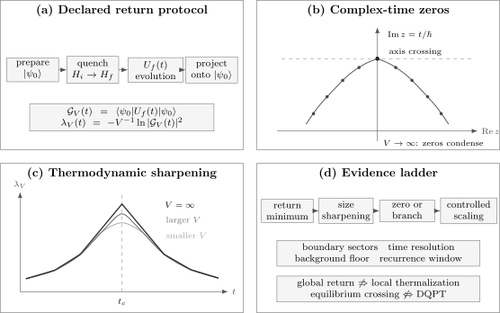
A DQPT claim needs a declared return quantity and size normalization. Complex-time zeros may approach the physical line as $V\to\infty$, producing a nonanalytic limiting rate. A finite-size dip or one sharp curve is only the beginning of the evidence ladder.

Spectral Representation

Let

$$H_f|n_f\rangle = E_n^f|n_f\rangle$$

and expand

$$|\psi_0\rangle = \sum_n c_n|n_f\rangle, \qquad p_n = |c_n|^2.$$

Then

$$\mathcal G_V(t) = \sum_n p_n e^{-iE_n^ft/\hbar}.$$

Thus the return amplitude is the characteristic function of the final-energy probability distribution. It depends on the diagonal weights $p_n$, not on relative phases among the $c_n$ in this energy basis. By contrast, a generic observable

$$\langle O(t)\rangle = \sum_{m,n} c_m^*c_n e^{i(E_m^f-E_n^f)t/\hbar} O_{mn}$$

also depends on energy-basis coherences and on the matrix elements of $O$. This already explains why a return-rate singularity need not appear in every local observable.

Energy-origin invariance

Changing the energy zero by

$$H_f \longmapsto H_f+C_V\mathbf 1$$

gives

$$\mathcal G_V(t) \longmapsto e^{-iC_Vt/\hbar} \mathcal G_V(t).$$

Therefore $\mathcal L_V(t)$ and $\lambda_V(t)$ are unchanged. The complex phase of $\mathcal G_V$ depends on the energy origin, but its zeros and squared magnitude do not.

Short-time baseline

The cumulant expansion begins as

$$\begin{aligned} \ln\mathcal G_V(t) &= -\frac{i\langle H_f\rangle_0t}{\hbar} \\ &\quad -\frac{(\Delta H_f)^2_0t^2}{2\hbar^2} +O(t^3). \end{aligned}$$

Consequently,

$$\lambda_V(t) = \frac{(\Delta H_f)^2_0}{V\hbar^2} t^2 +O(t^4).$$

For a state with an extensive energy variance, the intensive rate has a finite quadratic onset. A fitted cusp at times comparable to the sampling interval must first be distinguished from this analytic short-time law.

Why an Intensive Logarithm Is Needed

For many global quenches,

$$\mathcal L_V(t) \asymp e^{-V\lambda(t)}$$

over a suitable thermodynamic time window. The raw overlap is then exponentially small even when $\lambda(t)$ is ordinary and smooth. Dividing its logarithm by $V$ extracts an intensive object, just as an equilibrium free-energy density extracts the extensive logarithm of a partition function.

The analogy has limits:

• $\mathcal G(t)$ is generally complex, whereas an equilibrium partition function at real positive inverse temperature is positive;
• the initial state acts as a temporal boundary condition;
• time is not temperature;
• $\lambda(t)$ is a global large-deviation quantity, not an equilibrium thermodynamic potential;
• its singularities need not organize local static correlations in the same way as an equilibrium critical point.

The analogy is mathematically productive precisely when these differences remain visible.

Complex Time and the Boundary Partition Function

Introduce a complex variable $z$ with units of inverse energy:

$$\mathcal Z_V(z) = \langle\psi_0| e^{-zH_f} |\psi_0\rangle = \sum_n p_n e^{-zE_n^f}.$$

Physical real-time evolution lies on the imaginary-$z$ axis:

$$z = \frac{it}{\hbar}.$$

For a finite-dimensional lattice system, $\mathcal Z_V(z)$ is an entire function because it is a finite sum of exponentials. Define a complex boundary free-energy density on any zero-free patch by

$$f_V(z) = -\frac{1}{V} \operatorname{Log}\mathcal Z_V(z).$$

The logarithm requires a branch choice, but its real part on the physical line is unambiguous:

$$\lambda_V(t) = 2\operatorname{Re} f_V\!\left(\frac{it}{\hbar}\right).$$

For unbounded continuum Hamiltonians, convergence and domain questions must be checked before calling $\mathcal Z(z)$ entire. The finite-lattice construction is the clean reference case.

Fisher zeros

The zeros

$$\mathcal Z_V(z_j)=0$$

are called Fisher zeros by analogy with zeros of equilibrium partition functions in a complex temperature-like variable. At finite $V$, they are isolated unless a special factorization or degeneracy changes the structure. As $V$ grows, they can become dense on curves or regions.

A DQPT can occur when the thermodynamic accumulation set reaches the physical axis. Schematically,

$$\operatorname{Re}z_j(V) \longrightarrow 0, \qquad \hbar\operatorname{Im}z_j(V) \longrightarrow t_c.$$

The limiting free-energy branch then changes across $t_c$, and $\lambda(t)$ can become nonanalytic.

Zeros are sufficient structure, not a shortcut

Several cautions matter:

1. An exact zero can occur in a finite quantum system. That fact alone does not establish thermodynamic criticality.
2. A finite-size rate may be smooth because the nearest zero remains off the physical axis; its sharpening with size can still anticipate a DQPT.
3. A sharp analytic peak can arise when a zero line passes close to, but does not reach, the physical axis.
4. The thermodynamic singularity can be expressed as a crossing of dominant transfer-matrix branches even when directly locating every zero is impractical.
5. Experimental noise can prevent an observed probability from reaching zero while leaving a resolvable finite-size precursor.

The controlled statement is about the limiting analytic structure, not the visual drama of one trace.

Order of Limits

For fixed finite $V$, unitary dynamics is quasiperiodic when the spectrum is discrete. Recurrences are expected, and $\mathcal G_V(t)$ is analytic in $t$ even though it may have isolated real zeros. A thermodynamic DQPT instead concerns

$$\lambda(t) = -\lim_{V\to\infty} \frac{1}{V} \ln |\mathcal G_V(t)|^2$$

at fixed physical time.

The following operations need not commute:

$$\begin{aligned} &V\to\infty, &&t\to\infty, \\ &\delta t\to0, &&\text{noise strength}\to0. \end{aligned}$$

Taking $t\to\infty$ first at finite size probes recurrences and time averages. Taking $V\to\infty$ first can produce branch competition and real-time nonanalyticity. Convolving with finite time resolution before taking a derivative rounds a cusp. Removing noise after taking a logarithm can be singular if the inferred probability has crossed zero or a background floor.

A One-Qubit Zero Is Not a Phase Transition

Take

$$H = \frac{\hbar\Omega}{2} \sigma_z, \qquad |\psi_0\rangle = |{+x}\rangle.$$

Then

$$\begin{aligned} \mathcal G_1(t) &= \cos\!\left(\frac{\Omega t}{2}\right), \\ \mathcal L_1(t) &= \cos^2\!\left(\frac{\Omega t}{2}\right). \end{aligned}$$

The return probability vanishes at

$$t_n = \frac{(2n+1)\pi}{\Omega}.$$

This is exact destructive interference in a two-dimensional Hilbert space. There is no thermodynamic limit and therefore no many-body phase transition.

Now take $V$ independent copies:

$$H_V = \frac{\hbar\Omega}{2} \sum_{j=1}^{V} \sigma_j^z, \qquad |\Psi_0\rangle = |{+x}\rangle^{\otimes V}.$$

Factorization gives

$$\mathcal G_V(t) = \left[ \cos\!\left(\frac{\Omega t}{2}\right) \right]^V$$

and

$$\lambda(t) = -2\ln \left| \cos\!\left(\frac{\Omega t}{2}\right) \right|.$$

This thermodynamic rate is singular at the same times, even though the system is noninteracting and never entangles. The example is deliberately austere: a Loschmidt-rate DQPT does not by itself imply interactions, chaos, transport, thermalization, or spatial entanglement.

Exact Benchmark: Transverse-Field Ising Chain

Consider the periodic one-dimensional model

$$\begin{aligned} H(g) &= -J\sum_{j=1}^{V} \sigma_j^z\sigma_{j+1}^z \\ &\quad -Jg\sum_{j=1}^{V} \sigma_j^x, \\ &\text{with } J>0. \end{aligned}$$

The infinite chain has equilibrium quantum critical points at $g=\pm1$. For positive field, the familiar ordered-to-paramagnetic transition is at $g=1$. The canonical model conventions, parity sectors, and finite-size subtleties are developed in Transverse-Field Ising Model.

Prepare the ground state at $g_i$ and evolve after a sudden quench to $g_f$. A Jordan–Wigner transformation, Fourier transform, and Bogoliubov rotation reduce the even-parity problem to independent momentum pairs. The positive quasiparticle energy is

$$\epsilon_k(g) = 2J \sqrt{ 1+g^2-2g\cos k }.$$

It is useful to define the normalized pseudospin direction

$$\widehat{\mathbf d}_k(g) = \frac{ (\sin k,\,0,\,g-\cos k) }{ \sqrt{ \sin^2k+(g-\cos k)^2 } }.$$

The probability that the final $(k,-k)$ sector is in its excited pair state is

$$p_k = \frac{ 1- \widehat{\mathbf d}_k(g_i) \boldsymbol{\cdot} \widehat{\mathbf d}_k(g_f) }{2}.$$

Up to a nonzero analytic phase, the many-body return amplitude factorizes as

$$\mathcal G_V(t) \doteq \prod_{0<k<\pi} \left[ (1-p_k) +p_k e^{-2i\epsilon_k(g_f)t/\hbar} \right].$$

The symbol $\doteq$ indicates equality up to an overall phase that does not affect zeros or the return probability.

Mode-resolved return probability

For each momentum pair,

$$\begin{aligned} \mathcal L_k(t) ={}& \left| (1-p_k) +p_k e^{-2i\epsilon_k^ft/\hbar} \right|^2 \\ ={}& 1 -4p_k(1-p_k) \sin^2\!\left( \frac{\epsilon_k^ft}{\hbar} \right), \end{aligned}$$

where $\epsilon_k^f\equiv\epsilon_k(g_f)$. The thermodynamic rate is therefore

$$\begin{aligned} \lambda(t) &= -\int_0^\pi \frac{dk}{2\pi} \ln Q_k(t), \\ Q_k(t) &= 1 -4p_k(1-p_k) \sin^2\!\left( \frac{\epsilon_k^ft}{\hbar} \right). \end{aligned}$$

This formula displays the mechanism directly. A mode can become orthogonal to its initial state only if both conditions hold:

$$p_{k_*} = \frac12, \qquad \sin^2\!\left( \frac{\epsilon_{k_*}^ft}{\hbar} \right) = 1.$$

The first condition says that the quench populates the final two-level sector equally. The second says that its two amplitudes have accumulated a relative phase of $\pi$.

Critical momentum

The equal-population condition is

$$\widehat{\mathbf d}_{k_*}(g_i) \boldsymbol{\cdot} \widehat{\mathbf d}_{k_*}(g_f) = 0.$$

For the Ising chain this becomes

$$1+g_ig_f -(g_i+g_f)\cos k_* = 0,$$

so

$$\cos k_* = \frac{1+g_ig_f}{g_i+g_f}.$$

For $g_i,g_f>0$, a real $k_*\in(0,\pi)$ exists for a generic quench across $g=1$. This is the model-specific origin of the close relation between equilibrium and dynamical criticality in the original Ising-chain construction.

Critical times

At $k_*$ the critical times are

$$t_n^* = \left( n+\frac12 \right) \frac{\pi\hbar} {\epsilon_{k_*}^f}, \qquad n=0,1,2,\ldots.$$

The spacing is set by the post-quench energy of the critical mode, not directly by the equilibrium gap at $g=1$.

Fisher-zero lines

For complex $z$, a mode factor vanishes when

$$(1-p_k) +p_k e^{-2\epsilon_k^fz} = 0.$$

One convenient labeling of the zeros is

$$\begin{aligned} z_n(k) &= \frac{ \ln[p_k/(1-p_k)] +i\pi(2n+1) }{ 2\epsilon_k^f }, \\ n&\in\mathbb Z. \end{aligned}$$

As $k$ becomes continuous, these points form Fisher-zero lines. They cross the imaginary axis exactly when $p_{k_*}=1/2$. Substituting $z=it/\hbar$ then reproduces $t_n^*$.

Why a cusp appears

Near a simple critical mode and critical time, let

$$q = k-k_*, \qquad \tau = t-t_n^*.$$

After shifting $q$ to remove a mixed term, the argument of the logarithm has the generic local form

$$\mathcal L_k(t) \simeq Aq^2+B\tau^2, \qquad A,B>0.$$

The singular part of the one-dimensional momentum integral is therefore controlled by

$$-\int_{-\Lambda}^{\Lambda} dq\, \ln(Aq^2+B\tau^2).$$

Relative to its value at $\tau=0$, this contributes

$$\lambda_{\mathrm{sing}}(t) = -C|\tau| +o(|\tau|), \qquad C>0.$$

Thus a simple Fisher-line crossing produces a linear kink in one dimension. Other dimensions, dispersions, zero manifolds, and branch structures can produce different singular forms. The word “cusp” should not be promoted to a universal exponent without deriving the local zero geometry.

Finite-size momentum grids

At finite $V$, allowed momenta depend on fermion parity and spin boundary conditions. The continuum value $k_*$ is generally absent from the grid. Then $\mathcal L_V(t)$ remains nonzero near $t_n^*$ and $\lambda_V(t)$ is rounded. Its width narrows as the nearest allowed momentum approaches $k_*$.

Occasionally $k_*$ is exactly allowed, producing a real zero even at finite size. That arithmetic accident does not remove the need to compare size sequences and sectors. Boundary-condition averaging can help diagnose momentum-grid effects, but it must not be used to manufacture a smoother extrapolation without reporting the individual sectors.

What the Ising Result Does Not Generalize

The Ising-chain criterion is exact and illuminating, but several features are not universal:

• a quench across an equilibrium critical point need not produce a DQPT;
• a DQPT can occur for a quench whose endpoints lie in the same equilibrium phase;
• interacting and nonintegrable systems need not admit momentum-factorized amplitudes;
• critical times need not be periodic;
• a singularity need not come from one isolated quasiparticle momentum;
• a local order parameter need not vanish at a DQPT;
• finite temperature and dissipation do not have a unique extension of the pure-state definition.

Analyses of the XY and XXZ chains provide explicit counterexamples to a one-to-one equilibrium–dynamical correspondence. In transfer-matrix language, a nonanalyticity can appear when two leading boundary-transfer eigenvalues exchange dominance, regardless of whether the quench path crossed an equilibrium phase boundary.

Competing Exponential Branches

Suppose the initial Hamiltonian has a symmetry-broken ground-state manifold spanned by orthonormal states $|\psi_\alpha\rangle$. A physically natural return probability is

$$P_0(t) = \sum_{\alpha} \left| \langle\psi_\alpha| e^{-iH_ft/\hbar} |\psi_0\rangle \right|^2.$$

If each contribution has large-deviation form

$$P_\alpha(t) \asymp e^{-V\lambda_\alpha(t)},$$

then

$$\begin{aligned} \lambda_0(t) &= -\lim_{V\to\infty} \frac1V \ln P_0(t) \\ &= \min_\alpha \lambda_\alpha(t). \end{aligned}$$

The minimum of two analytic branches can have a cusp where their values cross. In a $\mathbb Z_2$-broken system, that crossing may coincide with a switch between positive- and negative-magnetization return sectors.

This mechanism was used in trapped-ion experiments: the two ferromagnetic reference probabilities were measured separately, and their branch exchange sharpened with size. The relation to magnetization is physically meaningful in that symmetry setting, but it is not a universal theorem for arbitrary DQPTs.

Branch crossings and finite systems

For finite $V$,

$$-\frac1V \ln \left( e^{-V\lambda_1} +e^{-V\lambda_2} \right)$$

is smooth when both probabilities are positive. Near the crossing, the rounding width is typically of order $1/V$ if the branch slopes differ. Replacing the sum by $\min(\lambda_1,\lambda_2)$ can expose the limiting kink in a small system, but this replacement is an asymptotic inference, not the measured finite-size rate itself.

Boundary Transfer Matrices

In one-dimensional tensor-network formulations, the return amplitude often takes the asymptotic form

$$\mathcal G_V(t) \simeq \sum_a c_a(t) \mu_a(t)^V,$$

where $\mu_a(t)$ are eigenvalues of a boundary transfer operator. Away from degeneracies, the eigenvalue with largest magnitude controls the rate:

$$\lambda(t) = -2\ln |\mu_{\max}(t)|.$$

If

$$|\mu_1(t_c)| = |\mu_2(t_c)|$$

and the dominant branch changes at $t_c$, the limiting rate can become nonanalytic. This is the dynamical counterpart of competing free-energy branches.

The transfer-matrix picture is especially useful for interacting chains because it does not require free quasiparticles. It also supplies a practical diagnostic: compare the leading complex eigenvalues, their magnitudes, and their convergence with bond dimension and time step.

Relation to Quantum Work

For a two-projective-measurement work protocol, the characteristic function is

$$\chi(u) = \left\langle e^{iH_i u/\hbar} e^{-iH_f u/\hbar} \right\rangle_0$$

for an initial state diagonal in the $H_i$ energy basis. If $|\psi_0\rangle$ is an $H_i$ eigenstate with energy $E_i$, then

$$\chi(u) = e^{iE_i u/\hbar} \mathcal G(u).$$

Therefore

$$|\chi(u)|^2 = \mathcal L(u)$$

for that preparation. The work distribution follows from the Fourier transform

$$P(W) = \frac{1}{2\pi\hbar} \int_{-\infty}^{\infty} du\, e^{-iuW/\hbar} \chi(u).$$

This relation connects return amplitudes, edge singularities of work distributions, and large-deviation theory. It does not identify work with an observable represented by one Hermitian operator, nor does it make every mixed-state work characteristic function equal to $\operatorname{Tr}[\rho_0e^{-iH_ft/\hbar}]$.

The phase factor $e^{iE_i u/\hbar}$ shifts the work origin but does not change the return probability or Fisher zeros. For a thermal initial state, the two-measurement protocol includes the initial energy distribution and generally differs from a naive interferometric trace unless the protocol is derived explicitly.

Equilibrium Criticality: Relation without Equivalence

The resemblance between

$$Z(\beta) = \operatorname{Tr}e^{-\beta H}$$

and

$$\mathcal Z(z) = \langle\psi_0|e^{-zH_f}|\psi_0\rangle$$

motivates the Fisher-zero construction, but the two objects have different boundary data. A useful comparison is:

Equilibrium transition	Loschmidt-rate DQPT
vary temperature or coupling	vary real time after a declared preparation
thermal trace or ground-state energy	boundary amplitude fixed by $\lvert\psi_0\rangle$
nonanalytic thermodynamic potential	nonanalytic return-rate density
thermodynamic state changes across control value	one state follows one unitary orbit
local order and correlations may have universal scaling	local signatures are model- and protocol-dependent

In the nearest-neighbor Ising-chain ground-state quench, crossing the equilibrium critical point produces an equal-population mode and hence DQPTs. In other models, the geometry of initial-state overlaps with final eigenvectors can permit or forbid Fisher-axis crossings independently of equilibrium phase labels.

The reliable statement is therefore conditional:

Equilibrium critical structure can constrain DQPTs in specific symmetry classes and protocols, but a DQPT is not a generic detector of equilibrium phase boundaries.

Order Parameters and Local Observables

A Loschmidt amplitude compares two vectors in the full Hilbert space. A local observable probes a reduced amount of information. Their thermodynamic scalings are different.

For a local operator $O_X$ with bounded support $X$, it is possible that

$$\lim_{V\to\infty} \langle O_X(t)\rangle$$

is smooth at $t_c$ while $\lambda(t)$ has a cusp. Conversely, a long-time order parameter can change nonanalytically as a Hamiltonian parameter is varied even if the Loschmidt rate has no real-time singularity.

Connections do occur in controlled settings:

• symmetry-manifold branch crossings can coincide with an order-parameter sign change;
• scaling near some DQPT fixed points can appear in correlation functions;
• momentum-resolved zeros can organize dynamical vortices in two-band systems;
• anomalous and regular cusp sequences in long-range Ising models can correlate with distinct order-parameter regimes.

Each connection requires its own assumptions. Measuring a magnetization zero near a return-rate peak is supporting evidence, not a replacement for the rate-function limit.

Dynamical Topological Order Parameters

For a translationally invariant two-band or Bogoliubov–de Gennes system, the return amplitude can factorize over momenta:

$$\mathcal G(t) = \prod_k \mathcal G_k(t), \qquad \mathcal G_k(t) = r_k(t)e^{i\phi_k(t)}.$$

Separate the phase into dynamical and geometric parts:

$$\phi_k^{\mathrm G}(t) = \phi_k(t) -\phi_k^{\mathrm{dyn}}(t),$$

with

$$\phi_k^{\mathrm{dyn}}(t) = -\frac1\hbar \int_0^t ds\, \langle\psi_k(s)| H_f(k) |\psi_k(s)\rangle.$$

Under boundary conditions that pin the geometric phase at the endpoints of a one-dimensional momentum interval, one can define a winding

$$\nu_D(t) = \frac{1}{2\pi} \int_0^\pi dk\, \partial_k \phi_k^{\mathrm G}(t).$$

At a critical mode where $\mathcal G_{k_*}(t_c)=0$, its phase is undefined and $\nu_D$ can jump by an integer. This is a dynamical topological order parameter.

The construction is powerful but not universal:

• it assumes a momentum-resolved factorization or an appropriate generalization;
• quantization depends on symmetries and endpoint conditions;
• it is distinct from the conserved topology of the instantaneously evolved many-body wavefunction;
• a DTOP jump does not imply that every equilibrium topological invariant changed;
• disorder, interactions, degeneracies, and mixed states require additional definitions.

Momentum-space tomography in cold-atom two-band systems has visualized phase vortices associated with such critical modes. Those vortices are a specialized, information-rich route to DQPT evidence, not the generic measurement protocol for an interacting spin system.

Interactions, Integrability, and Chaos

DQPTs occur in free, integrable, nonintegrable, and even product systems. Therefore:

$$\text{DQPT} \not\Rightarrow \text{integrability},$$

and

$$\text{DQPT} \not\Rightarrow \text{many-body chaos}.$$

Likewise, neither ETH nor level repulsion guarantees a Loschmidt-rate cusp. The return amplitude depends on a particular initial-state energy distribution and on coherent phase cancellation. Spectral statistics alone do not determine that distribution.

Weak integrability-breaking perturbations can shift or deform critical times and may preserve early DQPTs over accessible windows. At longer times, new branch crossings or rounded structures can appear. A claim of robustness should specify:

• the perturbation family;
• how its norm scales with $V$;
• the time interval tested;
• whether the thermodynamic limit was direct or extrapolated;
• which cusp property remained stable.

The same caution applies to long-range interactions. Kac normalization, interaction exponent, finite-size geometry, and order of limits can alter both equilibrium extensivity and dynamical branch structure.

Orthogonality Catastrophe and Local Quenches

The Anderson orthogonality catastrophe concerns the vanishing overlap of many-body ground states under a local perturbation as system size grows. A Loschmidt amplitude is instead time dependent and compares an initial state with its evolved image. The two ideas meet in local-quench problems, where boundary field theory and work-edge singularities can govern power-law decay.

For a local quench, however, the natural scaling may be subextensive:

$$-\ln\mathcal L_V(t) = o(V).$$

Then the volume-normalized rate satisfies

$$\lambda(t)=0$$

even though the overlap has nontrivial time dependence. One should choose the normalization dictated by the perturbation geometry rather than forcing every echo into a bulk DQPT framework.

Recurrences and Long Times

Finite isolated systems recur. A near-unity return at a late time does not invalidate earlier dephasing, and a sequence of small returns does not prove irreversibility.

The relevant windows are:

$$t_{\mathrm{micro}} \ll t \ll t_{\mathrm{recur}}(V),$$

with additional restrictions from boundary reflections, tensor-network convergence, and experimental coherence. DQPT critical times should be shown to stabilize inside a growing pre-recurrence window as $V$ increases.

Periodic critical times in an exactly factorized model are not generic recurrences of the full state. They arise from repeated destructive interference of a critical sector. Conversely, a finite-size revival peak can occur without any thermodynamic nonanalyticity.

Mixed States and Finite Temperature

For an initial density operator $\rho_0$, several plausible quantities coexist.

An interferometric amplitude is

$$\mathcal G_{\mathrm{int}}(t) = \operatorname{Tr} \left[ \rho_0e^{-iH_ft/\hbar} \right].$$

A fidelity return is

$$\mathcal L_F(t) = F\!\left( \rho_0, e^{-iH_ft/\hbar} \rho_0 e^{iH_ft/\hbar} \right),$$

where this site uses the squared Uhlmann-fidelity convention. Purification-based amplitudes, interferometric phases, and work-characteristic functions provide still other choices.

They agree in selected pure-state limits but differ at finite temperature. As a result, statements such as “temperature destroys the DQPT” or “the DQPT survives at finite temperature” are incomplete unless the return definition, preparation, and measured protocol are stated.

The conservative workflow is:

1. define the operational experiment;
2. derive the corresponding mathematical quantity;
3. specify the extensive normalization;
4. analyze its thermodynamic analytic structure;
5. compare other definitions only after identifying conditions for equivalence.

Open-System Extensions

Under a quantum channel $\mathcal E_t$, one might study

$$F\!\left( \rho_0, \mathcal E_t(\rho_0) \right),$$

a survival probability, a purification overlap, a trajectory generating function, or the spectrum of a tilted generator. These probe different physics.

Open-system dynamical phase transitions can also refer to:

• nonanalytic steady states of a Lindbladian;
• closing of a Liouvillian spectral gap;
• trajectory-space large-deviation transitions;
• exceptional points;
• transient singularities in a chosen generalized return.

None is automatically the closed pure-state DQPT defined at the start of this page. Cross-pollination is useful, but shared vocabulary is not equivalence.

Experimental Access

No single measurement architecture is optimal for every system.

Direct projective return

Prepare $|\psi_0\rangle$, evolve, and measure the projector

$$\Pi_0 = |\psi_0\rangle\langle\psi_0|.$$

Then

$$\langle\Pi_0\rangle_t = \mathcal L_V(t).$$

For a computational-basis product state, this may be one bit-string probability. For a degenerate reference manifold, sum the probabilities of the declared basis states.

The difficulty is sampling. If

$$\mathcal L_V(t) \sim e^{-V\lambda(t)},$$

then a Bernoulli estimator from $N_{\mathrm{shot}}$ repetitions has relative uncertainty approximately

$$\frac{\delta\mathcal L} {\mathcal L} \sim \frac{1} {\sqrt{ N_{\mathrm{shot}}\mathcal L }}$$

when $\mathcal L\ll1$. Fixed relative precision therefore requires exponentially many shots in the worst case.

Ancilla interferometry

A controlled evolution can encode

$$\operatorname{Re}\mathcal G(t) \quad\text{and}\quad \operatorname{Im}\mathcal G(t)$$

in an ancilla’s coherences. This gives phase information and can connect directly to work-characteristic measurements. Its cost is a controlled many-body evolution, plus careful calibration of ancilla dephasing and control phases.

Momentum-resolved tomography

For factorized two-band systems, reconstructing the Bloch vector of each momentum sector gives $\mathcal G_k(t)$, its phase, and dynamical vortices. This can locate critical modes without measuring an exponentially small full many-body probability. It depends strongly on translational invariance and an effectively Gaussian mode description.

Tensor-network and quantum-circuit transfer matrices

Infinite matrix product states can represent the thermodynamic state directly. Classical or quantum circuits can estimate a dominant transfer eigenvalue rather than a finite-chain overlap. This trades finite-size extrapolation for ansatz, bond-dimension, optimizer, sampling, and device-noise audits.

Landmark demonstrations

Platform	Quantity accessed	Main qualification
trapped-ion Ising simulator, 2017	returns to two ferromagnetic reference states for chains up to ten ions	finite-size branch analysis inferred the limiting kink
ultracold fermions in a driven optical lattice, 2018	momentum-resolved state tomography and dynamical vortices	specialized two-band topological setting
superconducting-qubit simulation, 2019	simulated momentum-sector dynamics and geometric phase	compact simulator of a factorized model
superconducting processor with an infinite-MPS-inspired circuit, 2022	transfer-eigenvalue cost through an Ising DQPT	ansatz and error mitigation replace ordinary finite-size scaling
trapped-ion processor with variational circuit MPS, 2026	variational thermodynamic-state evolution through an Ising DQPT	hybrid quantum–classical inference and sampling controls remain essential

These experiments establish several viable access routes. They do not remove the need to state which return object, effective model, normalization, and extrapolation each route realizes.

Noise, Resolution, and Background Floors

Suppose the measured probability is

$$\mathcal L_{\mathrm{meas}}(t) = (1-\eta) \mathcal L_{\mathrm{ideal}}(t) +\eta B(t),$$

where $B(t)$ is a background and $\eta$ summarizes preparation, measurement, or decoherence error. Near a deep minimum, even small $\eta$ can dominate. Taking a logarithm produces

$$\lambda_{\mathrm{meas}}(t) = -\frac1V \ln\mathcal L_{\mathrm{meas}}(t),$$

so subtracting a background after the logarithm is not equivalent to correcting probabilities before it.

Finite time resolution convolves the probability or signal with an instrument response. A cusp in the limiting rate can become a smooth peak. A credible analysis reports:

• the raw count model;
• SPAM calibration and uncertainty;
• the time-response function;
• whether corrections were applied before or after logarithms;
• sensitivity to background priors;
• bootstrap or likelihood intervals for $t_c$;
• the size range over which the inferred sharpening persists.

Finite-Size Evidence

A mature DQPT claim should use more than a visual cusp.

Rate-function sequence

Plot

$$\lambda_V(t) = -\frac1V \ln\mathcal L_V(t)$$

for several sizes with the same Hamiltonian normalization, boundary family, and time units. Track:

• pseudocritical time $t_c(V)$;
• peak or kink width $w(V)$;
• left and right local slopes;
• minimum return probability;
• sensitivity to interpolation and smoothing;
• recurrence and boundary-reflection times.

The limiting claim is strengthened when $t_c(V)$ converges, $w(V)$ shrinks, and the slope discontinuity stabilizes before recurrences.

Complex-zero sequence

When complex-time evaluation is available, locate the nearest zero $z_0(V)$ and test

$$\operatorname{Re}z_0(V) \longrightarrow 0, \qquad \hbar\operatorname{Im}z_0(V) \longrightarrow t_c.$$

The distance to the physical axis is often a cleaner rounding diagnostic than the height of a real-time peak. Numerical analytic continuation is ill-conditioned, however; directly evaluating $\mathcal Z(z)$ is preferable to continuing noisy real-time data.

Branch-spectrum sequence

For transfer-matrix methods, compare

$$\begin{gathered} |\mu_1(t)|, \qquad |\mu_2(t)|, \\ \Delta_\mu(t) = \ln \frac{|\mu_1(t)|}{|\mu_2(t)|}. \end{gathered}$$

A stable sign change of $\Delta_\mu$ at increasing bond dimension supports branch exchange. Convergence of the rate alone can hide a poorly resolved subleading spectrum.

Scaling hypotheses must be earned

A fit such as

$$t_c(V) = t_c+aV^{-\omega}$$

is a hypothesis, not a definition. The exponent $\omega$ depends on geometry, boundaries, and the singular mechanism. Report alternative fit windows and corrections rather than assigning an equilibrium critical exponent by analogy.

Numerical Methods

Exact diagonalization

Given final eigenpairs,

$$\mathcal G_V(t) = \sum_n p_n e^{-iE_n^ft/\hbar}.$$

Resolve all exact symmetries before interpreting size trends. Accidental mixing of momentum, parity, or particle-number sectors changes both $p_n$ and level structure.

For larger sparse systems, Krylov propagation can compute

$$|\psi(t)\rangle = e^{-iH_ft/\hbar}|\psi_0\rangle$$

and then its overlap with $|\psi_0\rangle$ without diagonalizing the full Hamiltonian.

Free-fermion determinants

Gaussian states permit determinant, Pfaffian, or mode-product formulas. These are efficient but convention-sensitive. Audit:

• Nambu doubling;
• occupied versus empty mode conventions;
• the factor of two in pair energies;
• fermion-parity sectors;
• branch choices for determinant logarithms;
• momenta at $k=0$ and $k=\pi$.

Compute $\ln\mathcal L$ as a sum of mode logarithms to avoid underflow.

Tensor-network evolution

Matrix product states can reach the thermodynamic limit directly or evolve long finite chains. Report:

• bond dimension and truncation threshold;
• time step and integrator;
• energy and norm drift;
• convergence of $\lambda(t)$ and transfer eigenvalues;
• whether entanglement growth ends the reliable window before or after $t_c$.

A sharp feature appearing exactly when the bond dimension saturates is a warning, not evidence.

Complex-time calculations

Imaginary components of $z$ generate unitary evolution; real components generate nonunitary filtering. Tensor norms can become extremely ill-conditioned. Stabilized transfer matrices, arbitrary precision, or direct root tracking may be required.

Never infer Fisher zeros by applying an unconstrained high-order analytic continuation to noisy sampled data without stability tests. Many distinct analytic functions agree within real-axis error bars and disagree dramatically off axis.

An Evidence Ladder

The following claims become progressively stronger:

1. Deep return minimum: the evolved state is nearly orthogonal to the reference state at one size.
2. Size-dependent sharpening: a candidate nonanalytic thermodynamic feature is visible.
3. Stable limiting time: pseudocritical times converge before recurrences.
4. Zero or branch mechanism: Fisher zeros approach the axis or dominant transfer branches exchange.
5. Robustness: the result survives controlled changes in boundaries, resolution, perturbations, and numerical cutoffs.
6. Observable connection: a separately measured local, topological, or entanglement diagnostic follows a derived model-specific relation.
7. Universality: a scaling form and exponents hold across a declared family with controlled corrections.

Do not jump from rung 1 to rung 7.

Interpretation Matrix

Observation	Supports	Does not establish by itself
$\mathcal L_V(t)$ is tiny	global distinguishability from the initial state	local relaxation or thermalization
exact finite-size zero	destructive interference at that size	thermodynamic nonanalyticity
sharpening $\lambda_V(t)$	candidate DQPT	universal scaling
Fisher zeros approach physical axis	analytic mechanism for a DQPT	singularity of every local observable
order parameter changes sign	symmetry-sector dynamics	Loschmidt-rate DQPT in general
DTOP jumps	topological winding in the stated mode construction	change of every equilibrium topological invariant
cusp survives weak perturbation	robustness over tested scales	generic nonintegrable universality
repeated cusps	coherent critical-time sequence	many-body recurrence or time-crystalline order

Common Mistakes

• Calling every overlap minimum a dynamical phase transition.
• Taking a thermodynamic logarithm without declaring the size variable.
• Forgetting that the thermodynamic limit precedes the analyticity test.
• Treating an isolated finite-size zero as sufficient evidence.
• Using “Loschmidt echo” without writing the formula.
• Confusing one-evolution return probability with imperfect reversal.
• Assuming that crossing an equilibrium critical point is necessary or sufficient.
• Inferring thermalization, chaos, or entanglement from a cusp.
• Assuming critical times must be equally spaced.
• Ignoring parity sectors and boundary-dependent momentum grids in the Ising chain.
• Losing the factor of two associated with $(k,-k)$ pair excitation.
• Taking the complex logarithm without tracking branches.
• Fitting a cusp after a tensor-network convergence window has ended.
• Subtracting an experimental background after taking the logarithm.
• Treating a DTOP as a universal order parameter for interacting systems.
• Calling a finite-temperature or open-system quantity “the” Loschmidt echo without an operational definition.
• Using equilibrium critical exponents in a finite-time collapse without deriving the scaling form.
• Confusing a DQPT sequence with recurrences, Floquet time order, or a long-time DPT-I transition.

Exercises

1. Invariance under an energy shift

Let

$$H_f' = H_f+C\mathbf1.$$

Show that $\mathcal G'(t)$ differs from $\mathcal G(t)$ only by a phase. Which DQPT data are invariant?

Solution

Because the identity commutes with $H_f$,

$$e^{-iH_f't/\hbar} = e^{-iCt/\hbar} e^{-iH_ft/\hbar}.$$

Hence

$$\mathcal G'(t) = e^{-iCt/\hbar} \mathcal G(t).$$

The return probability, rate function, real critical times, and complex zeros are unchanged because the multiplying exponential is never zero. The absolute phase of the amplitude changes and therefore requires a declared energy origin in an interferometric measurement.

2. Independent-spin return rate

For

$$H_V = \frac{\hbar\Omega}{2} \sum_{j=1}^{V}\sigma_j^z$$

and $|\Psi_0\rangle=|{+x}\rangle^{\otimes V}$, derive $\mathcal G_V(t)$ and $\lambda(t)$. Explain why its singularities do not diagnose interactions.

Solution

Each spin contributes

$$\langle +x| e^{-i\Omega t\sigma_z/2} |+x\rangle = \cos\!\left(\frac{\Omega t}{2}\right).$$

The product state and sum Hamiltonian factorize, so

$$\mathcal G_V(t) = \cos^V\!\left(\frac{\Omega t}{2}\right).$$

Therefore

$$\begin{aligned} \lambda(t) &= -\lim_{V\to\infty} \frac1V \ln|\mathcal G_V(t)|^2 \\ &= -2\ln \left| \cos\!\left(\frac{\Omega t}{2}\right) \right|. \end{aligned}$$

It diverges when $\Omega t/2=(n+1/2)\pi$. Yet the Hamiltonian contains no interactions and the state remains a tensor product at all times. The singularity records an extensive product of identical one-spin destructive-interference events.

3. Critical momentum in the Ising chain

Using

$$\widehat{\mathbf d}_k(g) \propto (\sin k,0,g-\cos k),$$

derive

$$\cos k_* = \frac{1+g_ig_f}{g_i+g_f}.$$

Show that for positive $g_i$ and $g_f$, a generic quench across $g=1$ gives $|\cos k_*|<1$.

Solution

The equal-population condition is orthogonality of the two normalized pseudospins. Normalization does not affect whether their dot product vanishes:

$$\begin{aligned} 0 ={}& \sin^2k +(g_i-\cos k)(g_f-\cos k) \\ ={}& 1+g_ig_f -(g_i+g_f)\cos k. \end{aligned}$$

Solving gives the stated expression. Suppose $0<g_i<1<g_f$. Define the difference $D$ between the two squared expressions. Then

$$\begin{aligned} D &= (g_i+g_f)^2 -(1+g_ig_f)^2, \\ D &= (1-g_i^2)(g_f^2-1) >0. \end{aligned}$$

Both numerator and denominator are positive, so the ratio lies strictly between zero and one. Interchanging $g_i$ and $g_f$ gives the same result.

4. Fisher zeros and critical times

For one Ising momentum pair, solve

$$(1-p) +p e^{-2\epsilon z} = 0$$

for its zeros. Determine when a zero lies on $z=it/\hbar$.

Solution

Rearranging,

$$e^{-2\epsilon z} = -\frac{1-p}{p}.$$

Taking all logarithm branches gives

$$-2\epsilon z = \ln\!\left(\frac{1-p}{p}\right) +i\pi(2m+1).$$

Relabeling the integer yields

$$z_n = \frac{ \ln[p/(1-p)] +i\pi(2n+1) }{ 2\epsilon }.$$

Its real part vanishes exactly when $p=1/2$. Equating its imaginary part to $t/\hbar$ gives

$$t_n = \left(n+\frac12\right) \frac{\pi\hbar}{\epsilon},$$

up to the equivalent labeling of positive and negative times.

5. Linear cusp from a critical mode

Show that

$$I(\tau) = \int_{-\Lambda}^{\Lambda} dq\, \left[ \ln(q^2+c^2\tau^2) -\ln q^2 \right]$$

has leading small-$|\tau|$ behavior $2\pi c|\tau|$.

Solution

Differentiate with respect to $a=c|\tau|>0$:

$$\frac{dI}{da} = \int_{-\Lambda}^{\Lambda} dq\, \frac{2a}{q^2+a^2} = 4\arctan\!\left(\frac{\Lambda}{a}\right).$$

As $a\to0^+$,

$$\frac{dI}{da} \longrightarrow 2\pi.$$

Since $I(0)=0$,

$$I(\tau) = 2\pi c|\tau| +O(\tau^2/\Lambda).$$

The return rate carries a minus sign in front of the momentum logarithm, so its singular contribution is proportional to $-|\tau|$ plus analytic background.

6. Return to a broken-symmetry manifold

Suppose

$$P_0(t) = e^{-V\lambda_+(t)} +e^{-V\lambda_-(t)}.$$

Show that the limiting rate is $\min(\lambda_+,\lambda_-)$. Estimate the rounding width near a transverse crossing where

$$\lambda_+(t)-\lambda_-(t) \simeq s(t-t_c), \qquad s\ne0.$$

Solution

Factor out the smaller exponential. If $\lambda_+<\lambda_-$,

$$\begin{aligned} \delta\lambda &= \lambda_--\lambda_+ >0, \\ -\frac1V\ln P_0 &= \lambda_+ -r_V, \\ r_V &= \frac1V \ln\!\left[ 1+e^{-V\delta\lambda} \right]. \end{aligned}$$

The correction $r_V$ vanishes as $V\to\infty$, and the other ordering is analogous. Thus the limit is the minimum.

Both branches contribute appreciably when

$$V|\lambda_+-\lambda_-| \lesssim1.$$

Using the linear crossing gives

$$|t-t_c| \lesssim \frac{1}{V|s|}.$$

Hence the finite-size crossover narrows as $1/V$ in this simple branch model.

7. Work characteristic function

Let $|\psi_0\rangle$ satisfy

$$H_i|\psi_0\rangle = E_i|\psi_0\rangle.$$

Starting from

$$\chi(u) = \langle\psi_0| e^{iH_i u/\hbar} e^{-iH_f u/\hbar} |\psi_0\rangle,$$

derive its relation to $\mathcal G(u)$. What information changes?

Solution

Acting to the left or right with the initial-energy exponential gives

$$\begin{aligned} \chi(u) &= e^{iE_i u/\hbar} \mathcal G(u), \\ \mathcal G(u) &= \langle\psi_0| e^{-iH_fu/\hbar} |\psi_0\rangle. \end{aligned}$$

The phase shifts the work distribution’s energy origin by $E_i$. It leaves $|\chi(u)|^2$, the zeros, and all Loschmidt critical times unchanged.

8. Design a finite-size DQPT audit

You are given noisy return-probability data for $V=8,10,12,14$. List a minimal analysis that can distinguish a candidate thermodynamic cusp from a sharp finite-size minimum.

Solution

A minimal defensible audit would:

1. compute $\lambda_V(t)=-V^{-1}\ln\mathcal L_V(t)$ from a probability-level noise model;
2. fit the candidate time, width, and left/right slopes with uncertainty for every $V$;
3. verify convergence under time-grid refinement and alternative local fit windows;
4. test whether the candidate time stabilizes while the width shrinks;
5. locate recurrence and boundary-reflection times and exclude contaminated data;
6. compare parity or boundary sectors if they alter the allowed momentum grid;
7. propagate SPAM and background-floor uncertainty before taking logarithms;
8. where possible, compute the nearest complex zero or leading transfer branches independently;
9. repeat after controlled small Hamiltonian perturbations and numerical-cutoff changes.

Four sizes may still be insufficient for an asymptotic exponent. The appropriate conclusion can be “finite-size precursor consistent with a DQPT” rather than a claimed thermodynamic singularity.

Research Status

Several statements are well established:

• the pure-state boundary amplitude and return-rate definition;
• Fisher-zero and transfer-branch mechanisms;
• exact DQPTs in free and integrable models;
• DQPTs and finite-size precursors in interacting simulators;
• the absence of a general one-to-one map to equilibrium phase boundaries;
• the non-implication of chaos, thermalization, or entanglement.

Active research includes:

• classification and universality in generic interacting dimensions;
• relations among DPT-I, DPT-II, confinement, and anomalous cusp families;
• robust operational definitions for mixed and open systems;
• how much local information a return-rate singularity constrains;
• topology beyond Gaussian momentum-factorized settings;
• scalable estimators that avoid exponentially rare global-return sampling;
• trustworthy quantum-processor advantage for interacting DQPT observables.

Results in the second list should be presented with model, symmetry, dimension, interaction range, preparation, and diagnostic attached.

Further Connections

• Quantum Quenches — preparation, energy weights, spreading, entanglement, and the return-amplitude entry point.
• Thermodynamic Limit — limit ordering, recurrences, and intensive quantities.
• Transverse-Field Ising Model — Hamiltonian, phases, parity sectors, and exact spectrum.
• Jordan–Wigner Transformation — canonical spin-to-fermion mapping.
• Quantum Phase Transitions — equilibrium critical scaling and its distinct control-parameter limit.
• Order Parameters — symmetry and finite-size order diagnostics.
• Work Distributions — two-measurement work statistics and characteristic functions.
• Fidelity — mixed-state convention ledger.
• Dynamical Phase versus Geometric Phase — phase separation behind dynamical topological winding.
• Relaxation and Thermalization — why global return decay and local ensemble agreement are distinct.
• Many-Body Quantum Chaos Preview — spectral and eigenvector diagnostics not implied by a DQPT.
• Scrambling and OTOCs Preview — operator-growth diagnostics distinct from return amplitudes.

References

• M. E. Fisher, “The nature of critical points,” in Lectures in Theoretical Physics, Vol. 7C, University of Colorado Press, 1965.
• A. Peres, “Stability of quantum motion in chaotic and regular systems,” Physical Review A 30, 1610–1615 (1984). doi:10.1103/PhysRevA.30.1610
• R. A. Jalabert and H. M. Pastawski, “Environment-independent decoherence rate in classically chaotic systems,” Physical Review Letters 86, 2490–2493 (2001). doi:10.1103/PhysRevLett.86.2490
• T. Gorin, T. Prosen, T. H. Seligman, and M. Žnidarič, “Dynamics of Loschmidt echoes and fidelity decay,” Physics Reports 435, 33–156 (2006). doi:10.1016/j.physrep.2006.09.003
• A. Silva, “Statistics of the work done on a quantum critical system by quenching a control parameter,” Physical Review Letters 101, 120603 (2008). doi:10.1103/PhysRevLett.101.120603
• A. Gambassi and A. Silva, “Large deviations and universality in quantum quenches,” Physical Review Letters 109, 250602 (2012). doi:10.1103/PhysRevLett.109.250602
• M. Heyl, A. Polkovnikov, and S. Kehrein, “Dynamical quantum phase transitions in the transverse-field Ising model,” Physical Review Letters 110, 135704 (2013). doi:10.1103/PhysRevLett.110.135704
• C. Karrasch and D. Schuricht, “Dynamical phase transitions after quenches in nonintegrable models,” Physical Review B 87, 195104 (2013). doi:10.1103/PhysRevB.87.195104
• F. Andraschko and J. Sirker, “Dynamical quantum phase transitions and the Loschmidt echo: a transfer matrix approach,” Physical Review B 89, 125120 (2014). doi:10.1103/PhysRevB.89.125120
• S. Vajna and B. Dóra, “Disentangling dynamical phase transitions from equilibrium phase transitions,” Physical Review B 89, 161105(R) (2014). doi:10.1103/PhysRevB.89.161105
• M. Heyl, “Dynamical quantum phase transitions in systems with broken-symmetry phases,” Physical Review Letters 113, 205701 (2014). doi:10.1103/PhysRevLett.113.205701
• M. Heyl, “Scaling and universality at dynamical quantum phase transitions,” Physical Review Letters 115, 140602 (2015). doi:10.1103/PhysRevLett.115.140602
• S. Vajna and B. Dóra, “Topological classification of dynamical phase transitions,” Physical Review B 91, 155127 (2015). doi:10.1103/PhysRevB.91.155127
• J. N. Kriel, C. Karrasch, and S. Kehrein, “Dynamical quantum phase transitions in the axial next-nearest-neighbor Ising chain,” Physical Review B 90, 125106 (2014). doi:10.1103/PhysRevB.90.125106
• J. C. Budich and M. Heyl, “Dynamical topological order parameters far from equilibrium,” Physical Review B 93, 085416 (2016). doi:10.1103/PhysRevB.93.085416
• B. Žunkovič, A. Silva, and M. Fabrizio, “Dynamical phase transitions and Loschmidt echo in the infinite-range XY model,” Philosophical Transactions of the Royal Society A 374, 20150160 (2016). doi:10.1098/rsta.2015.0160
• P. Jurcevic, H. Shen, P. Hauke, C. Maier, T. Brydges, C. Hempel, B. P. Lanyon, M. Heyl, R. Blatt, and C. F. Roos, “Direct observation of dynamical quantum phase transitions in an interacting many-body system,” Physical Review Letters 119, 080501 (2017). doi:10.1103/PhysRevLett.119.080501
• I. Homrighausen, N. O. Abeling, V. Zauner-Stauber, and J. C. Halimeh, “Anomalous dynamical phase in quantum spin chains with long-range interactions,” Physical Review B 96, 104436 (2017). doi:10.1103/PhysRevB.96.104436
• J. C. Halimeh and V. Zauner-Stauber, “Dynamical phase diagram of quantum spin chains with long-range interactions,” Physical Review B 96, 134427 (2017). doi:10.1103/PhysRevB.96.134427
• S. A. Weidinger, M. Heyl, A. Silva, and M. Knap, “Dynamical quantum phase transitions in systems with continuous symmetry breaking,” Physical Review B 96, 134313 (2017). doi:10.1103/PhysRevB.96.134313
• N. Fläschner, D. Vogel, M. Tarnowski, B. S. Rem, D.-S. Lühmann, M. Heyl, J. C. Budich, L. Mathey, K. Sengstock, and C. Weitenberg, “Observation of dynamical vortices after quenches in a system with topology,” Nature Physics 14, 265–268 (2018). doi:10.1038/s41567-017-0013-8
• N. Sedlmayr, M. Fleischhauer, and J. Sirker, “The fate of dynamical phase transitions at finite temperatures and in open systems,” Physical Review B 97, 045147 (2018). doi:10.1103/PhysRevB.97.045147
• M. Heyl, “Dynamical quantum phase transitions: a review,” Reports on Progress in Physics 81, 054001 (2018). doi:10.1088/1361-6633/aaaf9a
• X.-Y. Guo, C. Yang, Y. Zeng, Y. Peng, H.-K. Li, H. Deng, Y.-R. Jin, S. Chen, D. Zheng, and H. Fan, “Observation of a dynamical quantum phase transition by a superconducting qubit simulation,” Physical Review Applied 11, 044080 (2019). doi:10.1103/PhysRevApplied.11.044080
• T. Hashizume, I. P. McCulloch, and J. C. Halimeh, “Dynamical phase transitions in the two-dimensional transverse-field Ising model,” Physical Review Research 4, 013250 (2022). doi:10.1103/PhysRevResearch.4.013250
• J. Dborin, V. Wimalaweera, F. Barratt, E. Ostby, T. E. O’Brien, and A. G. Green, “Simulating groundstate and dynamical quantum phase transitions on a superconducting quantum computer,” Nature Communications 13, 5977 (2022). doi:10.1038/s41467-022-33737-4
• Y. Liu, S. Lv, Y. Meng, Z. Tan, E. Zhao, and H. Zou, “Exact Fisher zeros and thermofield dynamics across a quantum critical point,” Physical Review Research 6, 043139 (2024). doi:10.1103/PhysRevResearch.6.043139
• L. Gover, V. Wimalaweera, F. Azad, M. DeCross, M. Foss-Feig, and A. G. Green, “Fully optimised variational simulation of a dynamical quantum phase transition on a trapped-ion quantum computer,” Quantum 10, 2109 (2026). doi:10.22331/q-2026-05-20-2109

Summary

The Loschmidt amplitude is the characteristic function of the post-quench energy distribution for a pure initial state. Its squared magnitude is a global return probability, and its extensive logarithm defines the return-rate density.

A Loschmidt-rate DQPT is a nonanalyticity of that density after the thermodynamic limit. Fisher zeros approaching the physical complex-time axis, or equivalently competing transfer branches, provide the analytic mechanism. The transverse-field Ising chain makes the mechanism exact: a momentum sector with equal final-state populations becomes orthogonal at a sequence of critical times, producing a cusp after momentum integration.

The interpretation must remain disciplined. DQPTs are not equivalent to equilibrium phase transitions, local order-parameter transitions, thermalization, chaos, entanglement, or imperfect reversibility. Strong evidence combines a declared return quantity, size scaling, zero or branch diagnostics, numerical convergence, experimental error propagation, and only then model-specific connections to local or topological observables.