Integrability and Generalized Gibbs Ensembles Preview

An isolated integrable many-body system can dephase and settle to stationary local behavior without forgetting enough information to reach an ordinary Gibbs ensemble. Its obstruction is structural: besides energy and familiar symmetry charges, it carries an extensive hierarchy of local or quasilocal conserved quantities.

The generalized Gibbs ensemble, or GGE, is the corresponding memory ledger:

$$\boxed{ \begin{gathered} [H,Q_r]=0 \quad\Longrightarrow\quad \langle Q_r\rangle_t = \langle Q_r\rangle_0, \\ \rho_{\mathrm{GGE}} = \frac{1}{Z_{\mathrm{GGE}}} \exp\!\left( -\sum_r\lambda_r Q_r \right). \end{gathered} }$$

The multipliers $\lambda_r$ are fixed by the initial charge data. The formula is simple; identifying a physically meaningful and complete charge family is not.

A GGE is therefore neither a synonym for “nonthermal” nor a universal formula that works once enough operators are placed in an exponent. It is a model-dependent compressed description of late-time local data. Its validity must be tested against a declared observable class and a controlled thermodynamic and long-time limit.

Scope and Canonical Ownership

This page owns the nonequilibrium interface among:

• an extensive local or quasilocal conserved-charge hierarchy;
• equilibration without ordinary Gibbs thermalization;
• maximum-entropy construction of a GGE;
• the exact free-fermion mode-occupation example;
• charge locality, truncation, independence, and completeness;
• thermodynamic Bethe root densities as interacting stationary-state data;
• generalized eigenstate thermalization and the quench-action viewpoint;
• evidence standards, experiments, and integrability-breaking caveats.

Exact Solutions Preview owns the structural meaning of quantum integrability, coordinate Bethe ansatz, factorized scattering, transfer matrices, Yang–Baxter consistency, and equilibrium thermodynamic Bethe ansatz. XXZ Spin Chain owns the model-specific Bethe equations and phase diagram. This page uses those structures only to explain stationary states after a quench.

Quantum Quenches owns the preparation protocol and transient observable dynamics. Relaxation and Thermalization owns dephasing, diagonal ensembles, equilibration bounds, and the general evidence ledger. Eigenstate Thermalization Hypothesis owns conventional ETH in generic nonintegrable systems.

Prethermalization Preview owns parametrically long plateaus generated by approximate conservation laws. Generalized hydrodynamics appears below only as the spatially inhomogeneous continuation of local GGE reasoning.

What Integrability Changes

There is no context-free definition of quantum integrability that covers every finite system, lattice, continuum model, and quantum field theory. For translation-invariant lattice systems, a useful working signature is an extensive family

$$\left\{ Q_r^{(L)} \right\}_{r=1}^{R(L)}$$

such that

$$\begin{aligned} [H_L,Q_r^{(L)}] &=0, \\ [Q_r^{(L)},Q_s^{(L)}] &=0, \end{aligned}$$

with $R(L)$ growing with system size and with controlled locality as $L\to\infty$.

The locality requirement is essential. Every spectral projector of a finite nondegenerate Hamiltonian commutes with $H$, but declaring all projectors “integrals of motion” would make every finite matrix integrable and would say nothing useful about local physics.

Ordinary symmetry charges are not enough

A generic particle-number-conserving lattice Hamiltonian may have

$$[H,N]=0$$

without being integrable. Translation, parity, total spin, or a finite-dimensional Lie symmetry can organize exact sectors while leaving dynamics within each sector chaotic.

An integrable hierarchy is stronger. Schematically, a local charge has the form

$$Q_r^{(L)} = \sum_{j=1}^{L} q_{r,j},$$

where $q_{r,j}$ is a translate of a density supported on a finite number of nearby sites. A quasilocal charge permits tails whose norm decays sufficiently rapidly with distance. Precise norms and boundary corrections depend on the model.

Free and interacting integrability

For a quadratic model, normal-mode occupations provide transparent charges:

$$H = \sum_k \varepsilon_k n_k, \qquad [H,n_k]=0.$$

Interacting Bethe-ansatz models are not free models in disguise. Their quasiparticles acquire scattering phases, bound-state species, and state-dependent dressing. Integrability constrains many-body scattering and supplies conserved charges; it does not remove interaction effects.

Boundaries and sectors remain part of the claim

Periodic, twisted, and integrable open boundaries can support different commuting families. A generic boundary perturbation may break exact integrability even when the bulk Hamiltonian is unchanged. Ordinary symmetry sectors must also be resolved before level statistics or eigenstate comparisons are interpreted. Many-Body Quantum Chaos Preview owns the block construction, gap-ratio benchmarks, random-matrix classes, and finite-size crossover audit.

Thus “the XXZ chain is integrable” is shorthand for a specified Hamiltonian, coupling range, representation, and compatible boundary construction, not every deformation carrying the same informal model name.

Equilibration Without Ordinary Thermalization

Let

$$\rho(t) = e^{-iHt}\rho_0e^{iHt}.$$

For a discrete spectrum, the infinite-time average is the dephased state

$$\omega = \sum_E P_E\rho_0P_E,$$

where $P_E$ projects onto the full degenerate eigenspace of energy $E$. This is the exact energy-basis memory ledger.

The state $\omega$ generally contains exponentially detailed information. A statistical ensemble is useful when much of that information is invisible to a chosen family of local observables.

The stationary claim is local

Let $A$ be a fixed finite region as $L\to\infty$. A successful GGE claim may be formulated as

$$\lim_{L\to\infty} \operatorname{Tr} \left[ O_A \left( \omega_L-\rho_{\mathrm{GGE},L} \right) \right] = 0$$

for every bounded operator $O_A$ in the declared local class.

Equivalently, one may compare reduced states:

$$\left\| \omega_{A,L} - \rho_{\mathrm{GGE},A,L} \right\|_1 \longrightarrow 0.$$

Neither statement requires global trace-norm closeness. The exact diagonal ensemble can retain microscopic correlations and phase-space information that no compact GGE reproduces globally.

Generalized thermalization

It is useful to separate three claims:

Claim	Late-time comparison
equilibration	observables remain close to a stationary value for most late times
Gibbs thermalization	stationary local values agree with an energy-based Gibbs ensemble
generalized thermalization	stationary local values agree with a GGE built from a complete relevant charge family

An integrable system may satisfy the first and third while violating the second. Persistent finite-size oscillations or exact revivals can still prevent equilibration on the accessible system.

Constructing a Generalized Gibbs Ensemble

Suppose a commuting family $\{Q_r\}$ has prescribed expectations

$$q_r^{(0)} = \operatorname{Tr}(\rho_0Q_r).$$

Among density operators satisfying

$$\operatorname{Tr}(\rho Q_r) = q_r^{(0)},$$

the maximum-entropy state is found by varying

$$\begin{aligned} \mathcal L[\rho] &= -\operatorname{Tr}(\rho\ln\rho) \\ &\quad -\alpha \left[ \operatorname{Tr}(\rho)-1 \right] \\ &\quad -\sum_r\lambda_r \left[ \operatorname{Tr}(\rho Q_r) -q_r^{(0)} \right]. \end{aligned}$$

Stationarity gives

$$\ln\rho = -(1+\alpha)I -\sum_r\lambda_rQ_r,$$

and therefore

$$\begin{aligned} \rho_{\mathrm{GGE}} &= \frac{e^{-\sum_r\lambda_rQ_r}} {Z_{\mathrm{GGE}}}, \\ Z_{\mathrm{GGE}} &= \operatorname{Tr} e^{-\sum_r\lambda_rQ_r}. \end{aligned}$$

This is the same constrained-inference logic developed on Maximum Entropy Principle. Dynamics enters through the choice and initial values of the conserved constraints.

Matching identities

The multipliers solve

$$-\frac{\partial\ln Z_{\mathrm{GGE}}} {\partial\lambda_r} = \langle Q_r\rangle_{\mathrm{GGE}} = q_r^{(0)}.$$

For commuting charges, the Hessian is their covariance matrix:

$$\frac{\partial^2\ln Z_{\mathrm{GGE}}} {\partial\lambda_r\partial\lambda_s} = \operatorname{Cov}_{\mathrm{GGE}}(Q_r,Q_s).$$

Null directions indicate redundant constraints or singular limits. Near a regular solution, the covariance matrix controls how sensitively the multipliers respond to charge data.

Ordinary Gibbs states are special cases

If the only retained extensive constraint is energy,

$$Q_1=H, \qquad \lambda_1=\beta,$$

the GGE reduces to the canonical state. Including a finite number of symmetry charges gives a generalized canonical or grand-canonical ensemble, for example

$$\rho \propto \exp \left[ -\beta(H-\mu N) \right].$$

That construction is not by itself evidence of integrability. The distinctive integrable problem is an extensive local or quasilocal hierarchy.

Choosing the Charge Family

Writing every conserved operator in an exponent is neither necessary nor useful. A physically informative family should address four questions.

Conservation

Each exact charge must satisfy

$$[H,Q_r]=0$$

for the stated finite-size sequence and boundary conditions, up to explicitly controlled boundary terms.

Locality or quasilocality

Local observables can retain memory of extensive charges with local densities. Highly nonlocal projectors may encode the full diagonal ensemble but do not provide a useful thermodynamic compression.

Independence

If

$$Q_3=aQ_1+bQ_2+cI,$$

then its multiplier only reparameterizes the same state. Independence can mean linear, functional, or thermodynamic independence depending on the representation. The criterion must be stated rather than inferred from the number of symbols.

Completeness relative to local observables

A charge family is complete when its expectation values uniquely determine the stationary macrostate relevant to the declared local observables. Completeness is stronger than having many charges and weaker than reconstructing the exact global density operator.

This definition is deliberately operational:

$$\left\{ \langle Q_r\rangle \right\} \quad\Longrightarrow\quad \left\{ \langle O_A\rangle_{\mathrm{stationary}} \right\}$$

for the intended local class.

Worked Example: Free Fermions

Consider spinless fermions on a periodic lattice with

$$H = \sum_k \varepsilon_k n_k, \qquad n_k=c_k^\dagger c_k.$$

Every $n_k$ has eigenvalues $0$ and $1$ and commutes with every other occupation. Let

$$\zeta_k = \langle n_k\rangle_0.$$

The mode-occupation GGE is

$$\rho_{\mathrm{GGE}} = \frac{1}{Z} \exp \left( -\sum_k\lambda_kn_k \right).$$

Because the modes factorize,

$$\rho_{\mathrm{GGE}} = \bigotimes_k \rho_k,$$

with

$$\rho_k = \frac{ |0_k\rangle\langle0_k| + e^{-\lambda_k} |1_k\rangle\langle1_k| }{ 1+e^{-\lambda_k} }.$$

Matching $\langle n_k\rangle$ gives

$$\zeta_k = \frac{1}{e^{\lambda_k}+1},$$

so

$$\lambda_k = \ln \left( \frac{1-\zeta_k}{\zeta_k} \right).$$

The limiting values $\zeta_k=0$ or $1$ correspond to $\lambda_k=\pm\infty$ and pure mode factors.

Why an ordinary Gibbs state is insufficient

A grand-canonical Gibbs state predicts

$$\zeta_k^{\mathrm{Gibbs}} = \frac{1} {e^{\beta(\varepsilon_k-\mu)}+1}.$$

It has only two adjustable parameters, $\beta$ and $\mu$. A generic quench produces a function $k\mapsto\zeta_k$ that is not Fermi–Dirac. Matching total energy and number therefore leaves other mode-weighted observables incorrect.

Local correlators

For a translation-invariant Gaussian stationary state,

$$\langle c_i^\dagger c_j\rangle_{\mathrm{GGE}} = \frac{1}{L} \sum_k e^{ik(j-i)} \zeta_k.$$

All local Gaussian correlators follow from this two-point function by Wick reduction. Thus the conserved occupation profile determines the local reduced state.

In a quadratic quench, the momentum-space covariance evolves as

$$\Gamma_{kk'}(t) = e^{i(\varepsilon_k-\varepsilon_{k'})t} \Gamma_{kk'}(0).$$

Under suitable nondegeneracy and regularity conditions, oscillatory $k\ne k'$ contributions vanish from fixed-range real-space correlators in the long-time and thermodynamic limits. The stationary covariance retains

$$\Gamma_{kk} = \zeta_k.$$

This is dephasing, not loss of the conserved occupations.

Mode occupations and local charges

An individual $n_k$ is delocalized in real space. For a translation-invariant chain, its Fourier moments generate finite-range charges:

$$\begin{aligned} Q_m^{(c)} &= \sum_j \left( c_j^\dagger c_{j+m} + c_{j+m}^\dagger c_j \right), \\ Q_m^{(s)} &= -i\sum_j \left( c_j^\dagger c_{j+m} - c_{j+m}^\dagger c_j \right). \end{aligned}$$

In momentum space,

$$\begin{aligned} Q_m^{(c)} &= 2\sum_k \cos(mk)n_k, \\ Q_m^{(s)} &= 2\sum_k \sin(mk)n_k. \end{aligned}$$

When the Fourier data are complete, the occupation-profile GGE and the local-charge GGE are equivalent for local observables. This equivalence is model and regularity dependent; it should be demonstrated, not assumed.

Truncated GGEs

A truncated ensemble retains charges only up to range $m_{\max}$:

$$\begin{aligned} \rho_{\mathrm{tGGE}} &\propto \exp \left[ -\sum_{m=0}^{m_{\max}} \Lambda_m \right], \\ \Lambda_m &= \lambda_m^{(c)}Q_m^{(c)} + \lambda_m^{(s)}Q_m^{(s)}. \end{aligned}$$

For a fixed subsystem of length $\ell$, charges with range comparable to or modestly larger than $\ell$ can often approximate its reduced state well. This is an approximation statement with a convergence test, not a license to choose an arbitrary short list.

Degeneracy caveat

If $\varepsilon_k=\varepsilon_{k'}$, coherences within the degenerate subspace need not dephase. A complete stationary description may require conserved bilinears

$$c_k^\dagger c_{k'}$$

inside that subspace, or a basis that diagonalizes the initial covariance while respecting the Hamiltonian. Ignoring degeneracies can make an apparently reasonable occupation GGE fail.

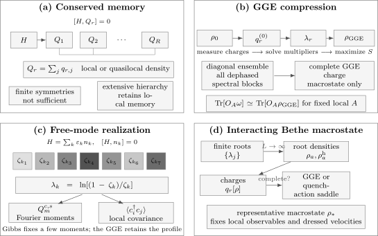
Integrable relaxation is a controlled compression problem. The diagonal ensemble keeps all dephased spectral data; a GGE keeps a complete local or quasilocal charge hierarchy. Free systems encode that hierarchy in mode occupations or their local Fourier moments, while interacting Bethe systems encode it in quasiparticle root densities.

Interacting Bethe-Ansatz Systems

In an interacting Bethe-ansatz model, a finite-density eigenstate contains a number of rapidities proportional to $L$. In the thermodynamic limit, microscopic roots are replaced by particle and hole densities

$$\rho_a(\lambda), \qquad \rho_a^{\mathrm h}(\lambda),$$

where $a$ labels quasiparticle species or bound-state strings and $\lambda$ is a rapidity.

The Bethe equations become constraints of the schematic form

$$\rho_a^{\mathrm t} = \rho_a+\rho_a^{\mathrm h} = a_a -\sum_b K_{ab}*\rho_b,$$

where

$$(K*f)(\lambda) = \int d\mu\, K(\lambda-\mu)f(\mu).$$

The kernels encode scattering. Their signs, normalizations, and species content are model dependent.

Conserved charges as functionals of root densities

An extensive charge density takes the form

$$q_r[\rho] = \sum_a \int d\lambda\, h_{r,a}(\lambda) \rho_a(\lambda),$$

where $h_{r,a}$ is the one-quasiparticle eigenvalue of charge $Q_r$. Matching the initial state means

$$q_r[\rho_*] = \lim_{L\to\infty} \frac{ \langle\psi_0|Q_r|\psi_0\rangle }{L}$$

for every charge in a complete family.

Unlike a free mode occupation, one root density influences dressed energies, velocities, and observables through coupled integral equations. The stationary macrostate is therefore an interacting thermodynamic object.

The generalized thermodynamic saddle

The number of microscopic Bethe states represented by smooth densities is controlled by the Yang–Yang entropy density

$$\begin{aligned} s_{\mathrm{YY}}[\rho] &= \sum_a\int d\lambda\, \big[ \rho_a^{\mathrm t}\ln\rho_a^{\mathrm t} \\ &\qquad -\rho_a\ln\rho_a -\rho_a^{\mathrm h}\ln\rho_a^{\mathrm h} \big]. \end{aligned}$$

A GGE macrostate extremizes

$$\mathcal I[\rho] = s_{\mathrm{YY}}[\rho] -\sum_r \lambda_rq_r[\rho]$$

subject to the Bethe constraints.

Define a generalized driving term

$$w_a(\lambda) = \sum_r \lambda_rh_{r,a}(\lambda).$$

In common fermionic TBA conventions, the saddle equations have the schematic form

$$\epsilon_a = w_a -\sum_b K_{ab}* \ln\!\left( 1+e^{-\epsilon_b} \right),$$

with filling

$$\vartheta_a = \frac{\rho_a}{\rho_a^{\mathrm t}} = \frac{1}{1+e^{\epsilon_a}}.$$

These equations show how a charge hierarchy becomes a stationary quasiparticle distribution. They are not a universal formula to transplant between models; bound-state content and kernel conventions must be rebuilt from the relevant Bethe equations.

Bethe ansatz preview

The nonequilibrium logic needs only three facts:

1. finite-volume eigenstates are labeled by interacting rapidities;
2. thermodynamic local physics is encoded by root-density functions;
3. a complete set of local and quasilocal charges must determine those functions.

The derivation of factorized scattering and the Bethe equations belongs to Exact Solutions Preview. The explicit spin-chain realization belongs to XXZ Spin Chain.

Generalized Eigenstate Thermalization

Conventional ETH proposes that local eigenstate expectation values are smooth functions of energy density and a finite set of symmetry densities. Integrable systems violate that compression: many macroscopically distinct root distributions can have the same energy density.

A generalized eigenstate-thermalization statement replaces energy by the complete integrable macrostate:

$$\langle n|O_A|n\rangle \longrightarrow \mathcal O_A[\rho]$$

for thermodynamic sequences of eigenstates whose root densities approach $\rho$.

Nearby microscopic Bethe states representing the same smooth $\rho$ then agree on local observables, while states at the same energy but with different $\rho$ need not agree.

This explains how one representative eigenstate can reproduce stationary local values in an integrable quench without satisfying conventional ETH. The “bath” for a small region is the rest of the system constrained by the full macrostate, not by energy alone.

The Quench-Action Viewpoint

For some interacting integrable quenches, initial-state overlaps with Bethe eigenstates are available in the thermodynamic limit. If

$$\left| \langle\{\lambda\}|\psi_0\rangle \right|^2 \asymp e^{-Lg_{\psi_0}[\rho]},$$

while the number of states near $\rho$ grows as

$$e^{Ls_{\mathrm{YY}}[\rho]},$$

then the dominant stationary macrostate minimizes the quench-action functional

$$\mathcal S_{\mathrm Q}[\rho] = g_{\psi_0}[\rho] -s_{\mathrm{YY}}[\rho]$$

subject to Bethe constraints.

The saddle $\rho_*$ supplies a representative state for local late-time observables. This construction uses more direct information about the initial overlaps than an initially guessed charge list.

The quench action and a complete GGE should identify the same local stationary macrostate when both apply. Disagreement is a diagnostic that the proposed GGE constraints are incomplete, incorrectly implemented, or outside their domain.

The Charge-Completeness Problem

The history of the XXZ chain provides an important warning.

Early GGEs used the familiar local charges generated by derivatives of a fundamental transfer matrix. For quenches involving bound-state strings, those charges did not uniquely determine every quasiparticle root density. Quench-action calculations and local correlators exposed the mismatch.

The lesson was not

$$\text{maximum entropy is invalid}.$$

It was

$$\begin{gathered} \text{the selected local charges} \\ \text{did not form a complete} \\ \text{macrostate coordinate system}. \end{gathered}$$

Quasilocal charge families associated with additional transfer-matrix representations supplied the missing information and led to complete GGEs for the spin-$1/2$ Heisenberg chain.

What “complete” does and does not mean

In this context, complete means sufficient to fix all thermodynamic root densities relevant to local observables. It does not mean:

• every bounded operator is included as a constraint;
• the exact finite-size diagonal ensemble is reconstructed;
• the same charge basis works for every integrable model;
• boundaries, degenerate sectors, or initial-state regularity can be ignored.

Completeness is a theorem or construction to establish model by model, not an adjective to attach to a long formula.

GGE Versus the Diagonal Ensemble

For a nondegenerate spectrum and pure initial state,

$$\rho_{\mathrm{diag}} = \sum_n |c_n|^2 |n\rangle\langle n|.$$

This ensemble exactly reproduces infinite-time averages of observables under the usual gap assumptions. It retains one population per eigenstate and is generally exponentially complex.

A GGE instead retains charge data:

$$\left\{ |c_n|^2 \right\}_{n=1}^{D} \quad\rightsquigarrow\quad \left\{ q_r^{(0)} \right\}_{r}.$$

The arrow is valid only for a chosen local observable class in a limit. It is not an equality of global states.

The comparison can be organized as follows:

Description	Memory retained	Exactness
time-evolved state	amplitudes and phases	exact unitary state
diagonal ensemble	dephased spectral blocks	exact infinite-time averages
complete GGE	relevant charge macrostate	exact or asymptotically exact for stated local observables
truncated GGE	finite subset of charges	controlled approximation only after convergence tests
Gibbs ensemble	energy and selected ordinary charges	generally insufficient in an integrable quench

How to Test a GGE Claim

A credible test should be designed before multipliers are fitted.

Step 1: Specify the model sequence

State:

• Hamiltonian and units;
• boundaries and twists;
• exact symmetry sector;
• system-size sequence;
• initial state or preparation protocol.

Step 2: Establish the integrable structure

Provide more than a small-size Poisson-like level-spacing plot. Useful structural evidence includes a free-mode mapping, complete Bethe construction, commuting transfer matrix, factorized scattering, or explicit extensive local and quasilocal charges.

Step 3: Declare the charge family

For each $Q_r$, state:

• its density or generating function;
• locality or quasilocality;
• normalization with $L$;
• boundary correction;
• independence and expected completeness.

Step 4: Compute initial charge data

Evaluate

$$q_r^{(0)} = \lim_{L\to\infty} \frac{\langle Q_r\rangle_0}{L}$$

analytically or with controlled numerical extrapolation. Conservation should be checked directly in finite calculations.

Step 5: Determine the stationary ensemble

Solve for $\lambda_r$, mode occupations, or Bethe root densities. Report regularization and truncation choices. In interacting models, positivity and Bethe constraints must be satisfied simultaneously.

Step 6: Reserve out-of-sample observables

Do not validate the GGE only on the charges used to fit it. Test:

• local correlators at several ranges;
• different operator species;
• subsystem reduced states where feasible;
• momentum distributions;
• currents or structure factors;
• finite-size and late-time trends.

Step 7: Compare competing descriptions

Place side by side:

$$\begin{gathered} \langle O\rangle_{\mathrm{time}}, \quad \langle O\rangle_{\mathrm{diag}}, \\ \langle O\rangle_{\mathrm{GGE}}, \quad \langle O\rangle_{\mathrm{Gibbs}}. \end{gathered}$$

Agreement of one fitted observable is not evidence. A complete claim needs a pattern across observables and sizes.

Step 8: Break integrability deliberately

Add a controlled perturbation and track whether:

• exact charge conservation is lost;
• a GGE-like plateau persists at intermediate times;
• late-time values drift toward ordinary Gibbs predictions.

This control separates an integrability mechanism from generic dephasing or finite-size trapping.

Experimental Evidence

Quantum Newton’s cradle

Kinoshita, Wenger, and Weiss prepared a nearly one-dimensional Bose gas whose momentum distribution remained strikingly nonthermal through thousands of collisions. The experiment established a prominent failure of rapid ordinary thermalization near an integrable regime.

It did not, by itself, reconstruct a complete GGE. Trapping, residual transverse excitations, finite observation time, and weak integrability breaking all matter. The correct conclusion is strong evidence for constrained dynamics, not a universal proof that any observed recurrence is integrability.

Correlations in split one-dimensional Bose gases

Langen and collaborators measured correlation functions up to high order after splitting a one-dimensional Bose gas and found agreement with a generalized ensemble built from approximately conserved mode data. This is substantially stronger than matching a single temperature-like quantity because higher-order correlators probe the distribution of fluctuations.

The inferred charges and effective low-energy model remain part of the experimental statement. A GGE is supported when one charge-calibrated description predicts additional observables, not merely when several free fit parameters can reproduce the same dataset.

Local GGEs and Generalized Hydrodynamics

A homogeneous GGE describes a stationary macrostate. In an inhomogeneous integrable system, each slowly varying cell can instead be approximated by a local GGE with root densities

$$\rho_a(x,t,\lambda).$$

At the Euler scale, generalized hydrodynamics transports each quasiparticle species according to

$$\partial_t\rho_a + \partial_x \left( v_a^{\mathrm{eff}}[\rho] \rho_a \right) = 0.$$

The effective velocity is dressed by the local state. This differs from ordinary hydrodynamics with only particle, momentum, and energy densities because the full quasiparticle distribution is a hydrodynamic field.

Diffusive corrections, external forces, integrability breaking, and fluctuating hydrodynamics require additional terms. The equation above is an interface, not a complete derivation.

Weak Integrability Breaking

Let

$$H = H_{\mathrm{int}} + gV, \qquad |g|\ll1,$$

where

$$[H_{\mathrm{int}},Q_r]=0.$$

Under the full Hamiltonian,

$$\frac{d}{dt} \langle Q_r\rangle = ig \langle[V,Q_r]\rangle.$$

The charges are no longer exact, but they can evolve slowly. A common sequence is

$$\begin{gathered} \text{microscopic dephasing} \\ \longrightarrow \text{GGE-like plateau} \\ \longrightarrow \text{ordinary thermalization}. \end{gathered}$$

The plateau lifetime is not universally $1/|g|$ or $1/g^2$. Selection rules, resonances, dimensionality, initial state, and the observable can change the scaling. The later prethermalization page owns these lifetime mechanisms.

Established Results and Active Boundaries

Well established

• Free and Gaussian integrable quenches often admit exact occupation-based GGEs for local observables.
• Interacting Bethe models require thermodynamic quasiparticle data rather than energy alone.
• Charge completeness is essential; a formally valid exponential with an incomplete charge set can predict wrong local correlators.
• Quasilocal charges are indispensable in important interacting chains.
• Integrable systems can equilibrate locally without ordinary Gibbs thermalization.
• Local GGEs are the thermodynamic building blocks of generalized hydrodynamics.

Model dependent

• which local and quasilocal charges form a complete family;
• whether a chosen initial state has a regular thermodynamic overlap functional;
• whether every target observable relaxes;
• how a truncated GGE converges with charge range;
• how boundaries and degeneracies alter the stationary algebra;
• the timescale on which weak perturbations destroy generalized thermalization.

Active or broader-frontier topics

• noncommuting and non-Abelian generalized ensembles;
• rigorous completeness beyond standard integrable chains;
• diffusive and fluctuating corrections to generalized hydrodynamics;
• kinetic theories of weak integrability breaking;
• integrability in higher dimensions and long-range systems;
• reconstruction of complete stationary data from experimentally accessible observables.

Common Mistakes

• Equating equilibration with Gibbs thermalization. Integrable systems may reach stationary local values that remain non-Gibbsian.
• Calling any finite collection of symmetries integrability. Particle number and translation alone do not form an extensive hierarchy.
• Using all spectral projectors as charges. That restates the diagonal ensemble and removes the locality that makes a GGE thermodynamic.
• Leaving the charge set unnamed. The symbol $\sum_r\lambda_rQ_r$ is not a prediction until the $Q_r$ are specified.
• Assuming local charges are automatically complete. Bound-state species can carry information missed by a familiar ultralocal hierarchy.
• Treating a failed charge list as a failure of maximum entropy. The constraints, not the variational principle, may be incomplete.
• Testing only fitted observables. Conserved charges agree by construction; reserve independent local probes.
• Ignoring degeneracies. Conserved coherences can survive within degenerate one-particle or many-body subspaces.
• Confusing free with integrable. Bethe-ansatz models can be strongly interacting.
• Expecting global-state agreement. A GGE normally targets local reduced states or few-body observables.
• Inferring integrability from persistent oscillations. Symmetry, weak coupling, finite-size recurrences, localization, or scars can mimic memory.
• Calling a prethermal GGE exact. Approximate charges drift under the full Hamiltonian.

A Compact Decision Ledger

Question	Ordinary Gibbs	GGE	Quench action
input data	energy and ordinary charges	complete relevant conserved charges	thermodynamic initial overlaps
natural variables	$\beta,\mu_a$	$\lambda_r$ or charge-generating functions	root-density saddle
free models	usually too coarse after a quench	often exact for local data	usually unnecessary
interacting Bethe models	generally too coarse	exact if charge family is complete	direct route when overlaps are known
global-state equality	no	no	no
main failure mode	omitted conserved memory	incomplete or ill-conditioned charges	unavailable or singular overlaps

Exercises

Exercise 1: Derive the generalized Gibbs form

Maximize

$$S(\rho) = -\operatorname{Tr}(\rho\ln\rho)$$

subject to normalization and

$$\operatorname{Tr}(\rho Q_r)=q_r.$$

Derive $\rho_{\mathrm{GGE}}$ and the matching identity for $\partial_{\lambda_r}\ln Z$.

Solution

Introduce

$$\begin{aligned} \mathcal L &= S(\rho) -\alpha \left[ \operatorname{Tr}(\rho)-1 \right] \\ &\quad -\sum_r\lambda_r \left[ \operatorname{Tr}(\rho Q_r)-q_r \right]. \end{aligned}$$

Using

$$\delta S = -\operatorname{Tr} \left[ \delta\rho(\ln\rho+I) \right],$$

stationarity for arbitrary Hermitian $\delta\rho$ gives

$$\ln\rho+I+\alpha I+\sum_r\lambda_rQ_r=0.$$

Hence

$$\rho = \frac{ e^{-\sum_r\lambda_rQ_r} }{Z}, \qquad Z = \operatorname{Tr} e^{-\sum_r\lambda_rQ_r}.$$

Differentiating under the trace and using cyclicity yields

$$-\partial_{\lambda_r}\ln Z = \operatorname{Tr}(\rho Q_r) = q_r.$$

Exercise 2: Solve one fermionic mode

For

$$\rho_k \propto e^{-\lambda_kn_k}, \qquad n_k^2=n_k,$$

derive the partition function, occupation, multiplier, and entropy in terms of $\zeta_k=\langle n_k\rangle$.

Solution

In the basis $\{|0\rangle,|1\rangle\}$,

$$Z_k = 1+e^{-\lambda_k}.$$

Therefore

$$\zeta_k = \frac{e^{-\lambda_k}} {1+e^{-\lambda_k}} = \frac{1}{e^{\lambda_k}+1},$$

so

$$\lambda_k = \ln \left( \frac{1-\zeta_k}{\zeta_k} \right).$$

The mode density matrix has eigenvalues $1-\zeta_k$ and $\zeta_k$, giving

$$S_k = -\zeta_k\ln\zeta_k -(1-\zeta_k) \ln(1-\zeta_k).$$

Exercise 3: Same energy and number, different memory

Consider four fermionic modes with energies

$$(-3,-1,1,3).$$

Compare occupation profiles

$$\boldsymbol\zeta_A = \left( \frac12,\frac12,\frac12,\frac12 \right)$$

and

$$\boldsymbol\zeta_B = (1,0,0,1).$$

Show that total number and energy agree, while

$$Q=n_1-n_2-n_3+n_4$$

distinguishes them.

Solution

Both profiles have

$$N = \sum_{a=1}^4\zeta_a = 2.$$

Their energies are

$$E_A = \frac12(-3-1+1+3) = 0$$

and

$$E_B = -3+3 = 0.$$

However,

$$\langle Q\rangle_A = 0, \qquad \langle Q\rangle_B = 2.$$

An ensemble constrained only by $E$ and $N$ cannot retain this distinction. A charge-complete GGE can.

Exercise 4: Show that Fourier charges are local

Using

$$c_j = \frac{1}{\sqrt L} \sum_k e^{ikj}c_k,$$

show that $Q_m^{(c)}$ and $Q_m^{(s)}$ are Fourier moments of $n_k$ and identify their real-space range.

Solution

Translation orthogonality gives

$$\sum_j c_j^\dagger c_{j+m} = \sum_k e^{ikm}n_k.$$

Adding the Hermitian conjugate yields

$$Q_m^{(c)} = 2\sum_k \cos(mk)n_k.$$

Taking the antisymmetric Hermitian combination gives

$$Q_m^{(s)} = 2\sum_k \sin(mk)n_k.$$

Each density connects sites separated by exactly $m$, so the charge has finite range $m$ even though each individual $n_k$ is delocalized.

Exercise 5: Detect an omitted local charge

Suppose $Q=\sum_jq_j$ is exactly conserved and the initial charge density is $q_0$. A proposed stationary ensemble predicts $q_{\mathrm{trial}}\ne q_0$. Explain why the ensemble cannot describe every local observable.

Solution

For a translation-invariant state,

$$\frac{\langle Q\rangle}{L} = \langle q_j\rangle.$$

Exact conservation fixes the left side to $q_0$. If the trial ensemble gives $q_{\mathrm{trial}}\ne q_0$, it already fails on the local density $q_j$. The mismatch cannot be repaired by taking a later time because $\langle Q\rangle$ is constant.

The conclusion requires $q_j$ to belong to the declared local observable class. A highly nonlocal conserved projector would not provide the same immediate local contradiction.

Exercise 6: Weakly break integrability

For

$$H=H_{\mathrm{int}}+gV, \qquad [H_{\mathrm{int}},Q_r]=0,$$

derive the exact rate of change of $\langle Q_r\rangle$ in units $\hbar=1$. Does the result prove a relaxation time proportional to $1/|g|$?

Solution

The Heisenberg equation gives

$$\frac{d}{dt} \langle Q_r\rangle = i\langle[H,Q_r]\rangle = ig\langle[V,Q_r]\rangle.$$

This shows that the instantaneous rate begins at order $g$ when the commutator expectation is nonzero. It does not prove a universal $1/|g|$ relaxation time. Oscillatory cancellations, selection rules, kinetic phase space, resonances, and higher-order processes can produce different scalings, including rates of order $g^2$ in suitable regimes.

Exercise 7: Why many charges can still be incomplete

An interacting Bethe model has two quasiparticle species with root densities $\rho_1(\lambda)$ and $\rho_2(\lambda)$. Suppose every charge in a proposed family depends only on

$$\rho_1(\lambda)+2\rho_2(\lambda).$$

Explain why the family need not determine local observables.

Solution

Different pairs $(\rho_1,\rho_2)$ can produce the same combination $\rho_1+2\rho_2$. The proposed charges therefore do not distinguish those macrostates.

If a local observable depends differently on the two species through dressing or form factors, its expectation values will differ even though every proposed charge agrees. Additional charges are needed whose one-particle eigenvalues resolve the species separately. This is the abstract structure behind charge-completeness problems involving Bethe strings.

Exercise 8: Design an out-of-sample GGE test

A numerical study fits $\lambda_r$ using energy, particle number, and three short-range charges, then reports agreement for those five quantities. Give a stronger validation protocol.

Solution

Agreement for fitted charges is automatic. A stronger protocol should:

1. compare against long-time and diagonal-ensemble values;
2. reserve local correlators not used in fitting, at several ranges;
3. test different operator species and, if feasible, a subsystem reduced state;
4. increase the retained charge range and verify convergence;
5. repeat over several system sizes and late-time windows;
6. compare with an ordinary Gibbs ensemble;
7. add a controlled integrability-breaking perturbation.

The study should also resolve exact symmetry sectors and report boundary conditions. This protocol tests predictive compression rather than parameter fitting.

Key Takeaways

• Integrable systems can equilibrate locally while retaining too much conserved information for an ordinary Gibbs state.
• A GGE is the maximum-entropy state constrained by a physically meaningful conserved-charge family.
• Locality, independence, and completeness are part of the construction, not optional refinements.
• Free fermions provide the exact model: mode occupations fix the GGE, while their Fourier moments form local charges.
• Interacting Bethe systems are encoded by thermodynamic quasiparticle root densities and dressed observables.
• A failed GGE often diagnoses an incomplete charge set; the XXZ history makes this distinction concrete.
• The diagonal ensemble is exact but exponentially detailed; a GGE is a local thermodynamic compression.
• Quench action uses initial overlaps to select the representative Bethe macrostate.
• Weak integrability breaking can produce a GGE-like plateau before ordinary thermalization.
• Evidence requires out-of-sample observables, finite-size control, and a declared charge basis.

Further Reading on This Site

• Nonequilibrium Overview for the chapter-wide map.
• Relaxation and Thermalization for diagonal ensembles and equilibration criteria.
• Eigenstate Thermalization Hypothesis for the nonintegrable comparison.
• Exact Solutions Preview for transfer matrices, factorized scattering, and thermodynamic Bethe ansatz.
• XXZ Spin Chain for the canonical interacting lattice example.
• Transverse-Field Ising Model for a quadratic spin-chain example.
• Maximum Entropy Principle for constrained inference.
• Time-Dependent Correlations for stationary and dynamical correlators.
• Transport Coefficients Preview for ballistic and diffusive response language.

References

1. E. T. Jaynes, “Information Theory and Statistical Mechanics,” Physical Review 106, 620–630 (1957). doi:10.1103/PhysRev.106.620
2. T. Kinoshita, T. Wenger, and D. S. Weiss, “A Quantum Newton’s Cradle,” Nature 440, 900–903 (2006). doi:10.1038/nature04693
3. M. Rigol, V. Dunjko, V. Yurovsky, and M. Olshanii, “Relaxation in a Completely Integrable Many-Body Quantum System,” Physical Review Letters 98, 050405 (2007). doi:10.1103/PhysRevLett.98.050405
4. T. Barthel and U. Schollwöck, “Dephasing and the Steady State in Quantum Many-Particle Systems,” Physical Review Letters 100, 100601 (2008). doi:10.1103/PhysRevLett.100.100601
5. M. Rigol, “Breakdown of Thermalization in Finite One-Dimensional Systems,” Physical Review Letters 103, 100403 (2009). doi:10.1103/PhysRevLett.103.100403
6. J.-S. Caux and J. Mossel, “Remarks on the Notion of Quantum Integrability,” Journal of Statistical Mechanics: Theory and Experiment 2011, P02023 (2011). doi:10.1088/1742-5468/2011/02/P02023
7. A. C. Cassidy, C. W. Clark, and M. Rigol, “Generalized Thermalization in an Integrable Lattice System,” Physical Review Letters 106, 140405 (2011). doi:10.1103/PhysRevLett.106.140405
8. P. Calabrese, F. H. L. Essler, and M. Fagotti, “Quantum Quench in the Transverse-Field Ising Chain,” Physical Review Letters 106, 227203 (2011). doi:10.1103/PhysRevLett.106.227203
9. M. Fagotti and F. H. L. Essler, “Reduced Density Matrix after a Quantum Quench,” Physical Review B 87, 245107 (2013). doi:10.1103/PhysRevB.87.245107
10. J.-S. Caux and F. H. L. Essler, “Time Evolution of Local Observables after Quenching to an Integrable Model,” Physical Review Letters 110, 257203 (2013). doi:10.1103/PhysRevLett.110.257203
11. B. Pozsgay, “The Generalized Gibbs Ensemble for Heisenberg Spin Chains,” Journal of Statistical Mechanics: Theory and Experiment 2013, P07003 (2013). doi:10.1088/1742-5468/2013/07/P07003
12. M. Fagotti, “On Conservation Laws, Relaxation and Pre-Relaxation after a Quantum Quench,” Journal of Statistical Mechanics: Theory and Experiment 2014, P03016 (2014). doi:10.1088/1742-5468/2014/03/P03016
13. B. Wouters, J. De Nardis, M. Brockmann, D. Fioretto, M. Rigol, and J.-S. Caux, “Quenching the Anisotropic Heisenberg Chain: Exact Solution and Generalized Gibbs Ensemble Predictions,” Physical Review Letters 113, 117202 (2014). doi:10.1103/PhysRevLett.113.117202
14. B. Pozsgay, M. Mestyán, M. A. Werner, M. Kormos, G. Zaránd, and G. Takács, “Correlations after Quantum Quenches in the XXZ Spin Chain: Failure of the Generalized Gibbs Ensemble,” Physical Review Letters 113, 117203 (2014). doi:10.1103/PhysRevLett.113.117203
15. G. Goldstein and N. Andrei, “Failure of the Local Generalized Gibbs Ensemble for Integrable Models with Bound States,” Physical Review A 90, 043625 (2014). doi:10.1103/PhysRevA.90.043625
16. E. Ilievski, J. De Nardis, B. Wouters, J.-S. Caux, F. H. L. Essler, and T. Prosen, “Complete Generalized Gibbs Ensembles in an Interacting Theory,” Physical Review Letters 115, 157201 (2015). doi:10.1103/PhysRevLett.115.157201
17. T. Langen, S. Erne, R. Geiger, B. Rauer, T. Schweigler, M. Kuhnert, W. Rohringer, I. E. Mazets, T. Gasenzer, and J. Schmiedmayer, “Experimental Observation of a Generalized Gibbs Ensemble,” Science 348, 207–211 (2015). doi:10.1126/science.1257026
18. F. H. L. Essler and M. Fagotti, “Quench Dynamics and Relaxation in Isolated Integrable Quantum Spin Chains,” Journal of Statistical Mechanics: Theory and Experiment 2016, 064002 (2016). doi:10.1088/1742-5468/2016/06/064002
19. L. Vidmar and M. Rigol, “Generalized Gibbs Ensemble in Integrable Lattice Models,” Journal of Statistical Mechanics: Theory and Experiment 2016, 064007 (2016). doi:10.1088/1742-5468/2016/06/064007
20. E. Ilievski, M. Medenjak, T. Prosen, and L. Zadnik, “Quasilocal Charges in Integrable Lattice Systems,” Journal of Statistical Mechanics: Theory and Experiment 2016, 064008 (2016). doi:10.1088/1742-5468/2016/06/064008
21. J.-S. Caux, “The Quench Action,” Journal of Statistical Mechanics: Theory and Experiment 2016, 064006 (2016). doi:10.1088/1742-5468/2016/06/064006
22. O. A. Castro-Alvaredo, B. Doyon, and T. Yoshimura, “Emergent Hydrodynamics in Integrable Quantum Systems Out of Equilibrium,” Physical Review X 6, 041065 (2016). doi:10.1103/PhysRevX.6.041065
23. B. Bertini, M. Collura, J. De Nardis, and M. Fagotti, “Transport in Out-of-Equilibrium XXZ Chains: Exact Profiles of Charges and Currents,” Physical Review Letters 117, 207201 (2016). doi:10.1103/PhysRevLett.117.207201
24. V. Alba and P. Calabrese, “Entanglement and Thermodynamics after a Quantum Quench in Integrable Systems,” Proceedings of the National Academy of Sciences 114, 7947–7951 (2017). doi:10.1073/pnas.1703516114
25. B. Doyon, H. Spohn, and T. Yoshimura, “A Geometric Viewpoint on Generalized Hydrodynamics,” Nuclear Physics B 926, 570–583 (2018). doi:10.1016/j.nuclphysb.2017.12.002