Scrambling and OTOCs Preview

Quantum information scrambling is the unitary delocalization of initially accessible information into many-body correlations, so that small output regions no longer suffice to recover it. An out-of-time-order correlator, or OTOC, is a four-point diagnostic of the accompanying Heisenberg-operator growth. It is powerful because it asks whether an initially local operator has become noncommuting with a distant probe. It is limited because one operator pair, one thermal ordering, and one experimental sequence do not by themselves establish recoverability, chaos, or thermalization.

Let

$$W_x(t) = e^{iHt/\hbar}W_xe^{-iHt/\hbar}$$

be the Heisenberg evolution of a bounded operator initially localized near $x$, and let $V_y$ be localized near $y$. A positive squared commutator is

$$\begin{aligned} A_{xy}(t) &= [W_x(t),V_y], \\ C_{WV}(x,y;t) &= \operatorname{Tr} \left[ \rho A_{xy}^\dagger(t)A_{xy}(t) \right]. \end{aligned}$$

It vanishes when the operators commute and grows as $W_x(t)$ acquires components that fail to commute with $V_y$. For unitary $W_x$ and $V_y$,

$$C_{WV}(x,y;t) = 2-2\operatorname{Re}F_{WV}(x,y;t),$$

where the unregularized OTOC is

$$F_{WV}(x,y;t) = \operatorname{Tr} \left[ \rho\, W_x^\dagger(t)V_y^\dagger W_x(t)V_y \right].$$

The operator order is not chronological: the sequence alternates between time $t$ and time $0$. That out-of-time ordering is what makes the correlator sensitive to noncommutativity generated by the dynamics.

The reliable inference chain is

$$\begin{gathered} \text{operator pair, state, and contour} \\ \longrightarrow \text{OTOC or commutator data} \\ \longrightarrow \text{front, rate, and saturation audit} \\ \longrightarrow \text{noise and finite-size controls} \\ \longrightarrow \text{qualified spreading claim}. \end{gathered}$$

No arrow should be silently replaced by the word chaos.

Purpose and Canonical Scope

This page is the canonical home for the dynamical and protocol-centered treatment of scrambling and OTOCs. It owns:

• unregularized, symmetrically regularized, and commutator-based thermal conventions;
• local operator growth from nested commutators;
• OTOC fronts, front broadening, and butterfly velocity;
• velocity-dependent growth or decay rates;
• the hierarchy among Lieb–Robinson, butterfly, entanglement, transport, and signal velocities;
• the assumptions behind a thermal Lyapunov exponent and the chaos bound;
• detection, decoding, and recoverability as distinct information tasks;
• echo, interferometric, randomized, two-copy, and teleportation protocols;
• model-by-model scrambling phenomenology;
• controlled links to quantum field theory, holography, and black holes;
• experimental and numerical evidence standards.

Neighboring pages retain separate canonical roles:

• Operator Entanglement and Scrambling Preview owns operator vectorization, operator Schmidt spectra, matrix-product-operator complexity, Pauli-string weights, Choi states, and tripartite information.
• Many-Body Quantum Chaos Preview owns symmetry-resolved level statistics, random-matrix universality, spectral form factors, and Thouless scales.
• SYK Model Preview owns the Majorana Hamiltonian, disorder variance, large-$N$ bilocal saddle, conformal and Schwarzian regimes, and finite-$N$ symmetry classes.
• Semiclassical Quantum Chaos Preview owns classical instability, trajectory sensitivity, Ehrenfest time, and semiclassical correspondence.
• Lieb–Robinson Bound owns the theorem, its norm estimates, and its locality assumptions.
• Eigenstate Thermalization Hypothesis owns the ETH ansatz and thermalization consequences.
• Time-Dependent Correlations owns ordinary response functions, spectral functions, and time-ordered correlators.
• Channel-State Duality owns the Choi construction and channel reconstruction.

Some operator-growth language must recur here so that the OTOC definitions are usable. The operator Schmidt decomposition and channel-state derivations are cross-linked rather than duplicated.

Epistemic Status

Established within stated settings

• A squared commutator exactly measures operator noncommutativity in the declared state or norm.
• Finite-range lattice Hamiltonians obey Lieb–Robinson-type upper bounds on commutator growth.
• Haar-random local circuits provide analytically controlled examples of ballistic fronts with broadening.
• Large-$N$ and semiclassical models can possess parametrically long exponential OTOC windows.
• Decoherence, imperfect reversal, and state-preparation errors can suppress a measured OTOC without unitary scrambling.
• Averaged OTOCs and channel-recovery quantities are related under explicit basis, state, and normalization choices.

Strongly supported but model dependent

• Generic one-dimensional nonintegrable local systems often exhibit a ballistic operator front.
• Quantum fluctuations often broaden that front, with diffusive broadening in important random-circuit and Hamiltonian examples.
• Conserved quantities leave hydrodynamic tails behind an otherwise ballistic front.
• Spectral chaos, ETH, operator growth, and entanglement growth commonly occur together in generic models.

Active or definition dependent

• The most universal front-shape classification for deterministic Hamiltonians;
• which regularization best represents a desired operational notion of thermal scrambling;
• precise relations among OTOC rates, transport coefficients, and entanglement velocities;
• robust thermodynamic extrapolation of Lyapunov windows from finite systems;
• universal fast-scrambling bounds under broad Hamiltonian and state assumptions;
• extracting intrinsic scrambling from noisy large-scale quantum processors.

The page therefore labels the observable, contour, state, operator family, scale, and limiting procedure before interpreting a result.

Assumptions and Convention Ledger

Unless stated otherwise:

• $H$ is a time-independent Hamiltonian generating closed-system unitary evolution;
• $W_x$ and $V_y$ are bounded local operators;
• $W_x(t)$ uses the Heisenberg convention shown above;
• thermal averages use

$$\rho_\beta = \frac{e^{-\beta H}}{Z}, \qquad Z = \operatorname{Tr}e^{-\beta H};$$

• infinite-temperature averages use $\rho_0=I/d$ in finite Hilbert space;
• the distance $r=d(x,y)$ is a graph or spatial distance declared with the model;
• $C_{WV}$ denotes the full positive squared commutator, whose maximum is $4$ for Hermitian unitaries;
• some literature instead calls $C_{WV}/2=1-\operatorname{Re}F_{WV}$ the squared commutator;
• logarithms are natural;
• the thermodynamic, large-$N$, long-time, and small-commutator limits are not interchanged without comment.

For fermionic odd operators, anticommutators or graded commutators may be the physically local objects. In gauge theories and continuum QFT, local algebras, smearing, ultraviolet regularization, and factorization require extra care.

OTOCs and Positive Commutator Norms

The algebraic identity

For unitary $W$ and $V$,

$$\begin{aligned} [W,V]^\dagger[W,V] &= 2I \\ &\quad -V^\dagger W^\dagger V W \\ &\quad -W^\dagger V^\dagger W V. \end{aligned}$$

The middle terms are adjoints. Taking an expectation value with any density operator gives

$$\begin{aligned} \left\langle [W,V]^\dagger[W,V] \right\rangle &= 2 \\ &\quad -2\operatorname{Re} \left\langle W^\dagger V^\dagger W V \right\rangle. \end{aligned}$$

This identity is exact and does not assume high temperature or chaos. What depends on the physical setting is the choice of state, operators, normalization, and thermal contour.

What the complex phase means

The positive commutator depends only on $\operatorname{Re}F$. The imaginary part can nevertheless carry information about operator ordering and nonlinear response. Reporting only $|F|$ discards both phase and sign; reporting only $\operatorname{Re}F$ does not reconstruct the full four-point function.

For Hermitian unitaries,

$$-1\leq \operatorname{Re}F\leq 1, \qquad 0\leq C\leq 4.$$

If nonunitary observables are used, the disconnected normalization and saturation scale are no longer fixed by these bounds. A normalized OTOC must then state its denominator explicitly.

State dependence

Three common choices answer different questions:

Average	Meaning	Main caution
$d^{-1}\operatorname{Tr}(\cdots)$	uniform operator-space average	finite-dimensional and effectively infinite temperature
$\operatorname{Tr}(\rho_\beta\cdots)$	thermal average	operator placement around the thermal circle matters
$\langle\psi	\cdots	\psi\rangle$

A state-resolved OTOC can be exactly the right observable. It should not be relabeled as a thermal Lyapunov diagnostic without demonstrating thermal typicality or performing the thermal average.

Thermal Ordering and Regularization

At nonzero temperature, cyclicity of the trace does not make all placements of $\rho_\beta$ equivalent. Moving an operator through the thermal density matrix shifts it in imaginary time through the Kubo–Martin–Schwinger relation. Distinct real-time contours can therefore produce distinct OTOCs.

Unregularized physical ordering

For Hermitian unitary probes, the most direct positive commutator uses

$$F_{\mathrm u}(t) = \operatorname{Tr} \left[ \rho_\beta W(t)V W(t)V \right],$$

and

$$C_{\mathrm u}(t) = 2-2\operatorname{Re}F_{\mathrm u}(t).$$

This quantity has an immediate noncommutativity interpretation. It can be ultraviolet sensitive for unbounded continuum operators, and it is not the particular analytic object used in the standard thermal chaos-bound argument.

Symmetric thermal-circle ordering

Define

$$y = \rho_\beta^{1/4}, \qquad y^4=\rho_\beta.$$

A symmetrically regularized four-point function is

$$F_{\mathrm{sym}}(t) = \operatorname{Tr} \left[ yV yW(t)yV yW(t) \right].$$

The four operators are evenly separated around the Euclidean thermal circle. This is the standard type of correlator entering the analytic chaos-bound framework. Its disconnected value and normalization must be computed with the same contour. In general,

$$F_{\mathrm{sym}}(t) \neq F_{\mathrm u}(t).$$

The difference can affect amplitudes and, in some weakly coupled field theories, the extracted growth spectrum itself. Symmetric regularization is therefore physical input, not a cosmetic numerical stabilizer.

A positive bipartite norm

Another useful regularized object is

$$\begin{aligned} C_{\mathrm b}(t) &= \operatorname{Tr} \left[ \rho_\beta^{1/2} [W(t),V]^\dagger \rho_\beta^{1/2} [W(t),V] \right] \\ &= \left\lVert \rho_\beta^{1/4} [W(t),V] \rho_\beta^{1/4} \right\rVert_2^2. \end{aligned}$$

It is manifestly nonnegative, but it is not generally equal to $2-2\operatorname{Re}F_{\mathrm{sym}}$. The diagonal terms also carry thermal insertions. This distinction is often hidden when all probes commute with $\rho_\beta$ or when the temperature is infinite.

The Contour Ledger

Before fitting any rate, record:

1. the exact operator sequence;
2. every power of $\rho_\beta$ between insertions;
3. whether operators are Hermitian or unitary;
4. the disconnected subtraction;
5. the normalization used at $t=0$ or late time;
6. whether the measured protocol realizes the same contour as the theory curve.

Two curves both called “the OTOC” need not be the same observable.

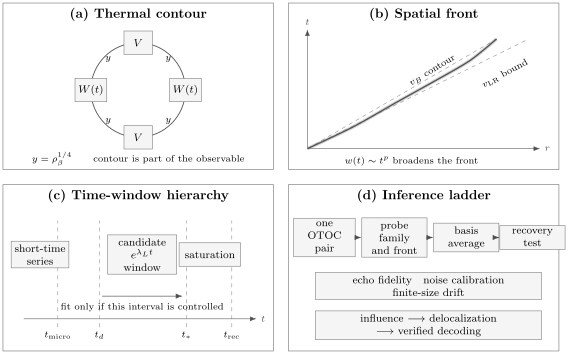
An OTOC claim has four independent ledgers. The thermal contour fixes the correlator; the spacetime profile fixes $v_B$ and front width; the time window determines whether a rate is meaningful; and the protocol hierarchy separates one operator-pair signal from verified information recovery. The Lieb–Robinson cone is an upper bound, not a measured butterfly front.

Local Operator Growth

Nested commutators

The Baker–Campbell–Hausdorff series gives

$$W_x(t) = \sum_{n=0}^{\infty} \frac{1}{n!} \left( \frac{it}{\hbar} \right)^n \operatorname{ad}_H^n(W_x),$$

where

$$\operatorname{ad}_H(W) = [H,W].$$

Suppose

$$H=\sum_X h_X$$

has interaction range $R$ on a lattice. Each commutator can enlarge support only through terms $h_X$ overlapping the current support. If $m$ interaction steps are required to connect $x$ to $y$, then

$$\left[ \operatorname{ad}_H^n(W_x),V_y \right] =0, \qquad n<m.$$

The commutator amplitude therefore begins no earlier than order $t^m$, and its squared norm no earlier than order $t^{2m}$. This is a microscopic statement about graph connectivity. It does not determine the late-time front speed, because path multiplicities, matrix elements, interference, and conservation laws enter at higher orders.

Support, weight, and complexity

An evolved operator can be expanded in an orthonormal local operator-string basis,

$$W(t) = \sum_{\mathcal S} c_{\mathcal S}(t)\mathcal S.$$

Several summaries are possible:

• support: the set of sites touched by strings with nonzero coefficient;
• site weight: the total $|c_{\mathcal S}|^2$ on strings acting nontrivially at a site;
• endpoint distribution: the weight whose rightmost or leftmost nonidentity factor is at a site;
• operator size: the number of elementary nonidentity factors in a string;
• operator entanglement: nonseparability of $W(t)$ across a cut.

A local OTOC probes a basis-dependent projection of this growth. Averaging over a complete local probe basis can recover a site-weight quantity at infinite temperature. One selected probe can miss operator components that commute with it.

The full derivations of string weights, operator size, and operator Schmidt spectra belong to Operator Entanglement and Scrambling Preview.

Rigorous Locality and the Butterfly Front

Lieb–Robinson control

For suitable short-range lattice Hamiltonians, a representative Lieb–Robinson estimate is

$$\left\lVert [W_x(t),V_y] \right\rVert \leq A \lVert W_x\rVert \lVert V_y\rVert e^{-\mu(r-v_{\mathrm{LR}}|t|)}.$$

The constants depend on the interaction graph and the chosen estimate. This establishes an exponentially small exterior region. It does not say that the physical front saturates the bound, and $v_{\mathrm{LR}}$ is generally not unique or sharp.

Because

$$C_{WV}(r,t) \leq \left\lVert [W_x(t),V_y] \right\rVert^2,$$

the same estimate bounds every state-averaged squared commutator. The converse fails: a small OTOC for one probe does not imply a small operator norm.

Operational butterfly velocity

Choose a threshold $0<C_\star<C_{\mathrm{sat}}$ and define the arrival time by

$$C_{WV}(r,t_\star(r)) = C_\star.$$

If

$$t_\star(r) = \frac{r}{v_B}+o(r),$$

then $v_B$ is the asymptotic butterfly velocity for that operator family, state, and threshold class. A trustworthy extraction checks that several thresholds converge to the same large-distance slope.

At finite size, the fitted value is an effective velocity. Boundary reflections, a short fitting baseline, and a changing front shape can produce threshold-dependent drift.

Front broadening

A useful scaling ansatz is

$$C(r,t) \simeq \Phi \left( \frac{r-v_B t}{w(t)} \right), \qquad w(t)\sim t^p.$$

The front is sharp on ballistic scales when $p<1$, but its absolute width still grows. Important cases include:

Exponent	Schematic behavior	Setting
$p=0$	asymptotically fixed width	idealized sharp-front or large-parameter limits
$p=1/2$	diffusive broadening	one-dimensional Haar-random circuits and related noisy-front descriptions
$p=1/3$	subdiffusive edge scaling	selected free or quasiparticle fronts
model dependent	nonuniversal broadening	deterministic, constrained, disordered, or long-range dynamics

These are classes of front behavior, not a lookup table proving chaos.

Velocity-dependent growth and decay

Along a spacetime ray $r=vt$, define, when the limit exists,

$$\lambda(v) = \lim_{t\to\infty} \frac{1}{t} \ln C(vt,t).$$

Outside a ballistic front,

$$\lambda(v)<0, \qquad v>v_B,$$

and the front is identified by

$$\lambda(v_B)=0.$$

Equivalently one can write

$$C(vt,t) \sim e^{-tI(v)}, \qquad I(v)=-\lambda(v)>0$$

outside the front. If

$$I(v) \sim a(v-v_B)^\alpha,$$

then a constant-$C$ contour has width

$$w(t) \sim t^{1-1/\alpha}.$$

Thus a quadratic rate function gives diffusive broadening.

In classical, semiclassical, or large-$N$ systems, a small commutator can grow exponentially for a parametrically long interval, allowing a positive interior rate. In a generic fully quantum local system with finite on-site dimension, $C(vt,t)$ usually saturates to order unity on interior rays. The strict long-time definition then gives $\lambda(v)=0$ inside, not a positive many-body Lyapunov exponent. A finite-window exponential fit and a ray-limit rate are different objects.

The Velocity Hierarchy

Several velocities can coexist in one model:

Symbol	What it tracks	What it does not establish
$v_{\mathrm{LR}}$	rigorous exterior norm bound	actual front position
$v_B$	an OTOC or commutator contour	entanglement production or transport rate
$v_E$	coarse entanglement-entropy growth	operator-norm causality
$v_g$	quasiparticle group velocity	generic interacting operator growth
$v_s$	sound propagation	diffusion or information recovery
$v_{\mathrm{sig}}$	an operational signaling protocol	a state-independent theorem bound

Often

$$v_B \leq v_{\mathrm{LR}},$$

but the right side depends on the chosen bound. Relations between $v_E$, $v_B$, diffusion constants, and sound speeds require model-specific assumptions. A diffusion constant has dimensions of length squared per time and is not itself a velocity.

Time Windows and Lyapunov Fits

Four distinct times

A rate claim should identify at least four scales:

1. Microscopic time $t_{\mathrm{micro}}$. Local interaction details and short-time series dominate.
2. Dissipation or local relaxation time $t_d$. Ordinary two-point functions have substantially relaxed.
3. Scrambling time $t_\ast$. The normalized connected OTOC correction becomes order unity.
4. Finite-size or recurrence time $t_{\mathrm{rec}}$. Discreteness, boundaries, or quasiperiodicity dominate.

In a controlled large-parameter regime, one may have

$$t_{\mathrm{micro}} \lesssim t_d \ll t \ll t_\ast \ll t_{\mathrm{rec}}.$$

Only the middle interval is a candidate for a clean exponential law.

Large-parameter growth

Suppose a normalized regularized correlator has the form

$$\frac{F_{\mathrm{disc}}-F(t)}{F_{\mathrm{disc}}} \simeq \frac{a}{\mathcal N_{\mathrm{eff}}} e^{\lambda_L t},$$

with $a$ of order unity and $\mathcal N_{\mathrm{eff}}\gg1$. Saturation occurs near

$$t_\ast \simeq \frac{1}{\lambda_L} \ln \mathcal N_{\mathrm{eff}}.$$

The logarithm is meaningful because the initial connected correction is parametrically small. In a small spin chain, an apparent straight segment on a semilog plot can instead be the crossover between a short-time power series and saturation.

A fit audit

For a claimed $\lambda_L$:

• fit the connected correction, not the full correlator with an arbitrary offset;
• vary the lower and upper endpoints of the window;
• compare exponential, power-law, and crossover models;
• propagate uncertainty in the disconnected normalization;
• repeat across sizes, temperatures, operator pairs, and regularizations;
• verify that the correction remains parametrically small throughout the fit;
• avoid fitting through front arrival when the observable is dominated by spatial propagation;
• report whether the rate is a local temporal rate, a velocity-dependent rate, or a global size-growth rate.

An exponential fit is evidence only when the window widens in the relevant limit.

The Thermal Chaos Bound

For a particular symmetrically regularized thermal four-point function satisfying analyticity, boundedness, factorization, and scale-separation assumptions, the Maldacena–Shenker–Stanford argument gives

$$\lambda_L \leq \frac{2\pi k_{\mathrm B}T}{\hbar}.$$

The statement concerns the growth rate of a small connected correction during a controlled interval. Its logic uses analyticity in a strip of complex time and a maximum-modulus-type bound.

The result does not directly bound:

• $v_B$ or any propagation velocity;
• an arbitrary unregularized OTOC;
• a rate fitted after saturation;
• classical Lyapunov exponents without the thermal analytic setup;
• open-system decay rates;
• nonthermal initial-state correlators;
• every finite-dimensional four-point function.

At infinite temperature the numerical upper bound diverges and becomes uninformative. At very low temperature the assumed window can disappear before a clean rate is observable. Saturation of the bound is a special dynamical property, not a definition of scrambling.

Strongly coupled large-$N$ Sachdev–Ye–Kitaev models and simple holographic black-hole regimes provide controlled examples approaching

$$\lambda_L = \frac{2\pi k_{\mathrm B}T}{\hbar}$$

in an appropriate limit. Generic short-range spin chains need not exhibit any parametrically long positive-$\lambda_L$ window.

Detection, Decoding, and Scrambling

Detection is the weaker task

Apply a small local perturbation near input region $A$, evolve with $U(t)$, and inspect an output region $D$. A local observable on $D$ can detect the perturbation only after the Heisenberg image of that observable overlaps the perturbation. Commutators and OTOCs quantify this influence for selected probes.

Detection asks:

$$\begin{gathered} \text{Can measurements on }D \\ \text{distinguish two inputs?} \end{gathered}$$

A nonzero OTOC commutator is therefore a witness of influence, not automatically a complete account of where the input quantum state can be recovered.

Decoding is the stronger task

To formulate recovery, entangle the input subsystem $A$ with a reference $R$, evolve the physical system, and ask which output region $D$ preserves the $R$ correlations. A decoder seeks a channel

$$\mathcal R_{D\to A'}$$

such that the recovered subsystem $A'$ is close to the original encoded state.

Strong scrambling means, in a declared code or ensemble:

• small output regions reveal little about $R$;
• the information has not been erased, because the global evolution is unitary;
• sufficiently large or suitably chosen output regions permit recovery;
• correlations are stored nonlocally across outputs.

This is why “locally inaccessible” is better than “lost.”

Why averaging matters

One OTOC samples one input perturbation and one output probe. Averaging over complete orthonormal operator bases on $A$ and $D$ can turn the family of OTOCs into a basis-independent channel quantity. Under explicit normalization choices, such averages are related to Rényi mutual information and decoupling diagnostics of the channel state.

The relationship is not automatic for:

• one hand-picked Pauli pair;
• an incomplete probe basis;
• a state-dependent normalization;
• a noisy nonunitary channel treated as if it were unitary;
• a postselected experiment without success-probability accounting.

The Choi-state and tripartite-information formulas are developed in Operator Entanglement and Scrambling Preview and Channel-State Duality.

A Two-Qubit Counterexample to Overinterpretation

Consider

$$H = JZ_1Z_2, \qquad W=X_1, \qquad V=X_2.$$

With

$$\theta = \frac{Jt}{\hbar},$$

the evolved operator is

$$W(t) = X_1\cos(2\theta) -Y_1Z_2\sin(2\theta).$$

Therefore

$$[W(t),X_2] = -2iY_1Y_2\sin(2\theta),$$

and every normalized state average gives

$$C(t) = 4\sin^2(2\theta).$$

The corresponding OTOC is

$$F(t) = \cos(4\theta).$$

The correlator reaches zero and becomes negative, yet the system has only two qubits and evolves periodically. The calculation demonstrates coherent operator growth and entangling dynamics. It does not establish thermodynamic chaos, irreversible scrambling, or thermalization.

Benchmark Dynamical Regimes

Haar-random local circuits

Brickwork circuits of independently Haar-random two-site gates provide an analytically controlled operator-hydrodynamic model. For local Hilbert-space dimension $q$, one common lattice convention gives an endpoint drift and diffusion coefficient

$$v_B = \frac{q^2-1}{q^2+1}, \qquad D_{\mathrm{end}} = \frac{2q^2}{(q^2+1)^2}.$$

The mean front moves ballistically while its width grows as

$$w(t) \sim \sqrt{D_{\mathrm{end}}t}.$$

The exact numerical coefficients depend on the circuit time-step and lattice-spacing convention. The robust lesson is the coexistence of ballistic drift and diffusive front broadening.

Random circuits are solvable universality laboratories. Their gate randomness is not required for every qualitative feature, but a result proved after a circuit average is not automatically a theorem for a deterministic Hamiltonian.

Conserved quantities

With a conserved density, operator weight splits into sectors. Nonconserved operator components can still advance ballistically, while the conserved component spreads diffusively and leaves a long hydrodynamic wake. Consequently:

• front arrival can be ballistic;
• approach to the interior saturation value can be algebraic;
• OTOCs involving the conserved density can differ sharply from generic probes;
• $v_B$ does not determine the diffusion constant.

This is one reason to use several operator families rather than one convenient Pauli component.

Free and integrable systems

Free quasiparticles can spread local operators ballistically. Selected squared commutators can grow, cross a front, and decay or saturate. Integrable interactions can generate complex operator strings while preserving an extensive charge structure.

Therefore:

$$\text{OTOC front} \not\Rightarrow \text{nonintegrability}.$$

Free fronts may display dispersive edge scaling, and integrable models can possess multiple characteristic velocities. The distinguishing evidence comes from conserved quantities, scattering structure, spectral statistics, and broader operator or recovery diagnostics.

Clifford dynamics

A Clifford circuit maps each Pauli string to a Pauli string. A Pauli OTOC can jump sharply when the evolved string begins to anticommute with a probe, even though the circuit remains efficiently classically simulable and lacks generic operator-amplitude complexity.

This example separates support growth from operator superposition growth. It also shows why a complete claim should include more than binary commutation data.

Localized and constrained dynamics

In many-body-localization phenomenology, dephasing among quasilocal conserved quantities produces a logarithmic operator light cone. OTOCs can reveal slow interaction-induced spreading even when particle or energy transport is strongly suppressed. Similar logarithmic behavior can also appear in certain disorder-free or noninteracting localized models, so the front alone does not certify an asymptotic MBL phase.

The status and avalanche caveats belong to Many-Body Localization Preview.

Long-range interactions

For interactions decaying as a power law, short-range exponential cones can be replaced by algebraic tails or modified cones. Direct couplings can produce early signals at long distance, and finite-system fits can mimic a very large velocity.

A long-range analysis must state:

• the decay exponent and spatial dimension;
• whether Kac normalization is used;
• the operator norm or state average being bounded;
• the asymptotic order of the distance and time limits;
• whether a linear cone is theoretically expected in that exponent regime.

There is no single $v_B$ formula covering every power-law model.

All-to-all and Sachdev–Ye–Kitaev dynamics

All-to-all models have no geometric butterfly cone. Operator size, rather than spatial radius, is the natural coordinate. In the Sachdev–Ye–Kitaev model, a simple fermion operator develops weight on products containing progressively more fermions. At large $N$, the early size and OTOC growth can be exponential, and the scrambling time scales logarithmically with $N$.

The SYK Model Preview declares the ensemble and derives the model-specific saddle, conformal propagator, Schwarzian mode, and finite-$N$ benchmark. This section retains the dynamical interpretation of its OTOC and operator-size growth.

This is the setting in which

$$t_\ast \sim \lambda_L^{-1}\ln N$$

is natural. A finite-range lattice of linear size $L$ must also move information across a physical diameter, giving a locality-controlled scale of order $L/v_B$. Calling both systems “fast scramblers” without naming the interaction graph conflates different problems.

Relation to Chaos, ETH, and Thermalization

The four notions are connected but inequivalent:

Observation	Supports	Does not alone prove
OTOC front	spatial operator influence	Wigner–Dyson statistics
extended exponential window	controlled instability of a declared correlator	global decoding or ETH
OTOC saturation	substantial noncommutativity for chosen probes	information recovery
ETH matrix elements	thermal behavior of local observables	a particular OTOC front law
level repulsion	spectral correlations in a symmetry sector	rapid scrambling
negative tripartite information	channel delocalization for a partition	a positive Lyapunov exponent

An OTOC is a four-point function. Written in the energy basis, it samples products of four operator matrix elements and several energy differences. The standard ETH ansatz constrains one- and two-eigenstate data but does not fully determine all correlations entering an OTOC. Higher-point ETH extensions address part of this gap.

Conversely, integrable and even classically nonchaotic models can show OTOC growth near unstable structures. Scrambling and chaos should therefore be named by diagnostic rather than treated as interchangeable labels.

Black-Hole and QFT Bridges

Shock-wave amplification

In simple holographic black-hole calculations, an early boundary perturbation creates a highly boosted bulk disturbance. Near the horizon, its effect can scale schematically as

$$G_{\mathrm N} e^{2\pi t/\beta},$$

where $G_{\mathrm N}$ supplies a small parameter. The corresponding boundary four-point function departs from factorization near

$$t_\ast \sim \frac{\beta}{2\pi} \ln\frac{1}{G_{\mathrm N}}.$$

In a holographic theory where entropy scales as $S\sim G_{\mathrm N}^{-1}$, this becomes the familiar logarithmic estimate

$$t_\ast \sim \frac{\beta}{2\pi}\ln S.$$

This controlled bridge motivates the language of butterfly effects and fast scrambling. It does not imply that a laboratory spin chain is a black hole, nor that every negative OTOC is evidence for gravity.

Relativistic microcausality

For local bosonic observables in a relativistic QFT,

$$[\mathcal O(x),\mathcal O(y)] =0$$

at spacelike separation. Thus the exact relativistic light cone is a causal exterior bound. Thermal OTOCs probe growth inside that cone and may define a butterfly velocity satisfying

$$v_B\leq c$$

in a suitable relativistic setting.

Continuum fields are unbounded operator-valued distributions. Coincident insertions can be ultraviolet singular, so operators should be smeared or regulated and the thermal contour declared. Lattice formulas cannot simply be pasted into QFT without these steps.

What is universal and what is not

The robust conceptual bridge is:

$$\begin{gathered} \text{local perturbation} \longrightarrow \text{operator growth} \\ \longrightarrow \text{loss of local recoverability}. \end{gathered}$$

The values of $\lambda_L$, $v_B$, $t_\ast$, front width, and saturation are theory dependent. Holographic saturation of a bound is a special large-$N$, strongly coupled result.

Measurement Protocols

Echo or time-reversal protocol

An echo sequence realizes the alternating operator order by combining forward and backward evolution. Schematically:

1. prepare $\rho$;
2. apply $V$;
3. evolve with $U(t)$;
4. apply $W$;
5. evolve with $U^\dagger(t)$;
6. measure a $V$-dependent observable.

The central challenge is implementing $U^\dagger(t)$, often by reversing the sign of the Hamiltonian. A reversal error can reduce the echo even in the absence of scrambling.

Ancilla interferometry

A control qubit can coherently select different operator orderings. Interference of the control branches yields the real or imaginary part of an OTOC. Controlled many-body operations and ancilla coherence are the principal costs.

Two-copy and thermofield protocols

Two copies can convert nonlinear functions of a density operator into measurable interference or swap observables. At finite temperature, a thermofield-double purification can realize thermal insertions on an enlarged Hilbert space. Preparation error in the purification changes the effective temperature and contour.

Randomized measurements

Randomized protocols prepare an ensemble of random local states or apply random basis rotations, evolve only forward, and infer OTOCs from cross-correlations of repeated measurement outcomes. They can avoid time reversal and ancillary controls. Their costs move into sampling, calibration of the random ensemble, and statistical postprocessing.

The inferred object depends on the unitary-design quality, subsystem size, and estimator normalization. A forward-only protocol is not automatically immune to decoherence.

Teleportation verification

Teleportation-based protocols embed the unknown input in entangled pairs, apply a scrambling unitary and its conjugate on two copies, and condition on a Bell-type projection. The teleportation fidelity supplies a positive recovery test, while the success probability or associated normalization helps separate coherent scrambling from nonscrambling noise.

This addresses a key false positive:

$$\begin{gathered} \text{OTOC decay from decoherence} \\ \neq \\ \text{unitary information delocalization}. \end{gathered}$$

The protocol itself has assumptions: copy matching, entangled-pair fidelity, postselection accounting, and a calibrated noise model.

Noise and False-Positive Controls

An experimental OTOC can decay because of:

• unitary operator growth;
• imperfect Hamiltonian reversal;
• dephasing or relaxation;
• leakage outside the computational subspace;
• readout and state-preparation errors;
• coherent control drift;
• mismatch between nominally identical copies;
• estimator bias and finite sampling.

A robust protocol includes several controls:

Control	What it diagnoses
identity or zero-time echo	state-preparation and measurement baseline
forward–backward fidelity	reversal quality
ordinary two-point correlators	local relaxation and dephasing scales
noninteracting or commuting benchmark	protocol-induced decay
deliberate noise injection	sensitivity of the estimator to decoherence
several operator pairs	probe-specific blind spots
size and distance scaling	front propagation versus global loss
teleportation or recovery fidelity	survival of encoded quantum information

The Decoherence Timescales page develops the open-system distinction in detail.

Experimental Status

Several platforms have measured OTOCs or closely related scrambling diagnostics:

• nuclear-magnetic-resonance simulators implemented echo-based local OTOC measurements;
• trapped-ion experiments measured collective OTOCs and later used randomized measurements in tunable long-range spin systems;
• ion-trap and superconducting qutrit processors implemented teleportation-based verification in small scrambling circuits;
• superconducting processors mapped information propagation, circuit scrambling, entanglement, and channel diagnostics;
• digital quantum computers have measured finite-temperature OTOCs using thermofield-double constructions.

These experiments establish control of increasingly sophisticated observables and distinguish several unitary and noisy mechanisms. They do not yet provide a platform-independent thermodynamic measurement of a universal Lyapunov exponent. Finite size, finite depth, connectivity, calibration, and protocol overhead remain part of every claim.

As of 2026, rigorous and operational speed-limit work continues to sharpen what “fast” means under different Hamiltonian and state assumptions. Those results complement rather than replace the contour- and protocol-specific OTOC analysis.

Numerical Workflow

Define the observable before evolving

Record:

• Hamiltonian, boundaries, and interaction graph;
• exact symmetries and state or ensemble;
• operator supports and algebra;
• thermal contour and normalization;
• whether the target is $F$, $\operatorname{Re}F$, $C$, a norm, or a basis average;
• intended order of limits.

Choose a method matched to the regime

Method	Strength	Main limitation
exact diagonalization	exact finite-system correlator	exponentially small sizes
Krylov time evolution	sparse Hamiltonians and selected states	finite-time and finite-size limits
typicality sampling	thermal traces without full diagonalization	stochastic and low-temperature cost
MPO evolution	one-dimensional operator fronts	bond dimension grows with operator entanglement
tensor-network folding	tailored spacetime contractions	geometry- and contour-dependent cost
random-circuit analytics	controlled ensemble averages	may not transfer quantitatively to Hamiltonians
semiclassical or kinetic theory	large occupation or weak coupling	approximation and regularization dependence

Map the full spacetime profile

Compute $C(r,t)$ over a window large enough to see:

1. the short-time nested-commutator onset;
2. the leading tail;
3. several front contours;
4. the interior approach to saturation;
5. boundary reflections or finite-size recurrences.

Fitting only the contour with the cleanest appearance hides threshold drift.

Convergence checks

For tensor networks, vary bond dimension and truncation tolerance separately inside, at, and outside the front. Tiny exterior tails are especially vulnerable to absolute truncation error. For exact or Krylov methods, vary timestep, Krylov dimension, precision, and system size. For stochastic traces, report sample variance and validate against exact traces at smaller size.

Inference ladder

A reproducible report should separate:

$$\begin{gathered} 1:\ \text{one operator-pair OTOC} \\ 2:\ \text{front geometry across probes} \\ 3:\ \text{basis-averaged channel test} \\ 4:\ \text{decoding or recovery test} \\ 5:\ \text{chaos or thermalization evidence} \end{gathered}$$

Each level adds information; none can be retroactively inferred from a lower level without extra assumptions.

Common Mistakes

• Calling every four-point function an OTOC without writing its operator order.
• Using $F_{\mathrm u}$ in numerics and comparing its rate directly with a bound derived for a symmetric contour.
• Forgetting whether the squared commutator is $C$ or $C/2$.
• Treating $F=0$ as maximum scrambling; for Hermitian unitaries, $F=-1$ gives $C=4$.
• Inferring operator-norm locality from one state-averaged OTOC.
• Equating $v_B$ with $v_{\mathrm{LR}}$, $v_E$, a group velocity, or a diffusion constant.
• Fitting an exponential across the short-time series, front arrival, and saturation crossover.
• Ignoring the disconnected subtraction or fitting its uncertainty as signal.
• Calling OTOC decay “information loss” under closed unitary evolution.
• Ignoring decoherence and imperfect reversal in an experiment.
• Treating an integrable or Clifford front as proof of many-body chaos.
• Importing large-$N$ or holographic conclusions into a small local spin chain without a controlled limit.
• Claiming a thermodynamic velocity from one small system and one threshold.
• Using unsmeared continuum fields at coincident points without a UV prescription.

Exercises

1. OTOC–commutator identity

Let $W$ and $V$ be unitary. Prove

$$\begin{aligned} \left\langle [W,V]^\dagger[W,V] \right\rangle &= 2 \\ &\quad -2\operatorname{Re} \left\langle W^\dagger V^\dagger WV \right\rangle. \end{aligned}$$

Which part of the complex OTOC is absent from the positive commutator?

Solution

Expand the product:

$$\begin{aligned} [W,V]^\dagger[W,V] &= V^\dagger W^\dagger WV \\ &\quad -V^\dagger W^\dagger VW \\ &\quad -W^\dagger V^\dagger WV \\ &\quad +W^\dagger V^\dagger VW. \end{aligned}$$

Unitarity makes the first and last terms equal to $I$. The two middle operators are adjoints, so their expectation values are complex conjugates. Hence

$$\begin{aligned} \langle[W,V]^\dagger[W,V]\rangle &= 2-F-F^\ast \\ &= 2-2\operatorname{Re}F. \end{aligned}$$

The imaginary part of $F$ is not determined by the positive squared commutator.

2. Exact two-qubit growth

For

$$H=JZ_1Z_2, \qquad W=X_1, \qquad V=X_2,$$

derive $W(t)$, $C(t)$, and $F(t)$. Explain why the result is not evidence for thermodynamic chaos.

Solution

Because $Z_1Z_2$ anticommutes with $X_1$ and squares to $I$,

$$\begin{aligned} e^{i\theta Z_1Z_2} X_1 e^{-i\theta Z_1Z_2} &= X_1\cos(2\theta) \\ &\quad -Y_1Z_2\sin(2\theta), \end{aligned}$$

where $\theta=Jt/\hbar$. Only the second term fails to commute with $X_2$, giving

$$[W(t),X_2] = -2iY_1Y_2\sin(2\theta).$$

Therefore

$$C(t) = 4\sin^2(2\theta),$$

and the unitary identity gives

$$F(t) = 1-\frac{C(t)}{2} = \cos(4\theta).$$

The motion is exactly periodic in a four-dimensional Hilbert space. It shows coherent operator spreading across one interaction edge, but there is no thermodynamic limit, sustained exponential window, irreversible relaxation, or random-matrix inference.

3. Graph distance and early-time power

Let $H$ be a nearest-neighbor Hamiltonian on a chain. Operators $W_0$ and $V_r$ are supported on sites $0$ and $r>0$. Show that the amplitude $[W_0(t),V_r]$ has no contribution below order $t^r$.

Solution

The $n$th term in the Heisenberg series is $\operatorname{ad}_H^n(W_0)$. One nearest-neighbor commutator can enlarge the support by at most one site. Therefore

$$\operatorname{supp} \operatorname{ad}_H^n(W_0) \subseteq \{-n,\ldots,n\}.$$

For $n<r$, this support does not reach site $r$, so

$$\left[ \operatorname{ad}_H^n(W_0),V_r \right]=0.$$

The commutator series starts no earlier than $n=r$, hence its amplitude is $O(t^r)$ and its positive squared norm is $O(t^{2r})$. Additional symmetries or cancellations can delay the first nonzero term.

4. Rate function and front width

Suppose outside the front

$$C(r,t) \sim \exp\left[ -at \left( \frac{r}{t}-v_B \right)^\alpha \right],$$

with $a>0$ and $\alpha>1$. Find the width of a fixed-$C$ contour around $r=v_Bt$.

Solution

Write

$$r = v_Bt+\delta r.$$

Then

$$t \left( \frac{r}{t}-v_B \right)^\alpha = \frac{(\delta r)^\alpha}{t^{\alpha-1}}.$$

A fixed value of $C$ requires this combination to remain constant, so

$$\delta r \sim t^{(\alpha-1)/\alpha} = t^{1-1/\alpha}.$$

For $\alpha=2$, the width scales as $t^{1/2}$.

5. Velocity inference

A simulation finds $v_B=1.3Ja/\hbar$ and a published Lieb–Robinson estimate gives $v_{\mathrm{LR}}=7Ja/\hbar$. Another calculation finds an entanglement velocity $v_E=0.8Ja/\hbar$. Which conclusions are justified?

Solution

The data are consistent with the rigorous exterior bound because $v_B<v_{\mathrm{LR}}$. The large gap does not imply that the numerical front is inaccurate; Lieb–Robinson estimates are often nonsharp. The fact that $v_E<v_B$ says that the chosen entropy-growth rate is slower than the chosen operator front in this setup. It does not establish a universal inequality unless the assumptions of a relevant theorem are checked. None of the three numbers determines a diffusion constant or a spectral-chaos class.

6. Is the exponential window controlled?

For system sizes $L=10,12,14$, an OTOC correction is well fit by $Ae^{\lambda t}$ over intervals of widths $0.8$, $0.9$, and $0.85$ in units of $J^{-1}$. The fitted $\lambda$ is stable. Is this enough to claim a many-body Lyapunov exponent?

Solution

No. A stable slope over a window that does not widen can be a finite crossover. One should test whether the connected correction is parametrically small, whether the interval separates from the microscopic and saturation scales, whether alternative power-law or crossover fits are disfavored, and whether a relevant large parameter produces an expanding interval. One must also state the thermal contour and check operator and temperature dependence. The stable fit is useful evidence, but not yet a controlled asymptotic exponent.

7. Design a decoherence control

An echo experiment observes $|F(t)|$ decay. Give a minimal set of measurements that can distinguish unitary scrambling from reversal error and decoherence.

Solution

A minimal control set includes:

1. a forward–backward echo with the scrambling insertion removed, to measure reversal fidelity;
2. ordinary one- and two-point observables, to estimate relaxation and dephasing times;
3. a commuting or noninteracting benchmark executed with the same pulse depth;
4. several spatially separated operator pairs, to test front propagation;
5. an independently calibrated noise model or deliberate noise scan;
6. a recovery-sensitive observable, such as teleportation fidelity, if the claim is information scrambling rather than operator noncommutativity.

A correction obtained by dividing two decaying signals must propagate denominator uncertainty and be validated on known circuits.

8. Local versus all-to-all scrambling time

Compare a one-dimensional short-range chain of length $L$ with an all-to-all model containing $N$ degrees of freedom. Why can $t_\ast\sim\ln N$ be natural in the second model but incomplete in the first?

Solution

In an all-to-all model, operator size can grow multiplicatively: an operator of size $s$ can interact with order $s$ new degrees of freedom, producing exponential size growth and $t_\ast\sim\lambda^{-1}\ln N$.

In a one-dimensional finite-range chain, locality restricts the advancing boundary. Information must cross a distance of order $L$, so global scrambling cannot occur before a scale of order

$$t_{\mathrm{cross}} \sim \frac{L}{v_B}.$$

Local complexity can grow behind the front, but the logarithmic size-growth estimate alone omits the geometric crossing time.

Key Takeaways

• An OTOC is a declared four-point function; a squared commutator is a positive noncommutativity diagnostic.
• Thermal operator placement matters. Unregularized, symmetric, and bipartite objects are generally different.
• Nested commutators explain the earliest graph-distance dependence; Lieb–Robinson bounds control an exterior region.
• The butterfly velocity is extracted from asymptotic OTOC contours and is not the Lieb–Robinson, entanglement, group, or transport velocity.
• A positive Lyapunov window is controlled only when it lies between distinct microscopic and scrambling scales and widens in a relevant limit.
• The thermal chaos bound applies to a specific regularized analytic setup, not to arbitrary decay curves.
• One OTOC establishes influence for one operator pair. Scrambling as information delocalization is stronger and ultimately concerns recovery.
• Decoherence and reversal error can mimic OTOC decay; verified protocols add independent recovery and noise diagnostics.
• Free, integrable, Clifford, localized, long-range, random-circuit, and large-$N$ systems can all spread operators in different ways.
• Black-hole and QFT links are precise within their controlled regimes and should remain qualified outside them.

Further Connections

• Nonequilibrium Overview places scrambling among relaxation, transport, and entanglement growth.
• Mutual Information in Many-Body Systems develops the correlation quantities used in recovery tests.
• Thermal Density Operators fixes ensemble and temperature conventions.
• Heisenberg Picture supplies the operator equation of motion.
• Commutators and Anticommutators reviews the algebra underlying squared-commutator identities.
• Thermodynamic Limit explains why finite-size saturation and asymptotic scrambling statements must be separated.
• Why Many-Body Quantum Mechanics Leads to QFT develops the continuum bridge without assuming holography.
• SYK Model Preview supplies the all-to-all Majorana model behind the controlled large-$N$ example.

References

• A. I. Larkin and Y. N. Ovchinnikov, “Quasiclassical method in the theory of superconductivity,” Soviet Physics JETP 28, 1200–1205 (1969).
• E. H. Lieb and D. W. Robinson, “The finite group velocity of quantum spin systems,” Communications in Mathematical Physics 28, 251–257 (1972). doi:10.1007/BF01645779
• P. Hayden and J. Preskill, “Black holes as mirrors: quantum information in random subsystems,” Journal of High Energy Physics 2007, 120 (2007). doi:10.1088/1126-6708/2007/09/120
• Y. Sekino and L. Susskind, “Fast scramblers,” Journal of High Energy Physics 2008, 065 (2008). doi:10.1088/1126-6708/2008/10/065
• S. H. Shenker and D. Stanford, “Black holes and the butterfly effect,” Journal of High Energy Physics 2014, 67 (2014). doi:10.1007/JHEP03(2014)067
• P. Hosur, X.-L. Qi, D. A. Roberts, and B. Yoshida, “Chaos in quantum channels,” Journal of High Energy Physics 2016, 4 (2016). doi:10.1007/JHEP02(2016)004
• J. Maldacena, S. H. Shenker, and D. Stanford, “A bound on chaos,” Journal of High Energy Physics 2016, 106 (2016). doi:10.1007/JHEP08(2016)106
• D. A. Roberts and B. Swingle, “Lieb–Robinson bound and the butterfly effect in quantum field theories,” Physical Review Letters 117, 091602 (2016). doi:10.1103/PhysRevLett.117.091602
• B. Swingle, G. Bentsen, M. Schleier-Smith, and P. Hayden, “Measuring the scrambling of quantum information,” Physical Review A 94, 040302(R) (2016). doi:10.1103/PhysRevA.94.040302
• J. Maldacena and D. Stanford, “Remarks on the Sachdev–Ye–Kitaev model,” Physical Review D 94, 106002 (2016). doi:10.1103/PhysRevD.94.106002
• J. Li et al., “Measuring out-of-time-order correlators on a nuclear magnetic resonance quantum simulator,” Physical Review X 7, 031011 (2017). doi:10.1103/PhysRevX.7.031011
• M. Gärttner et al., “Measuring out-of-time-order correlations and multiple quantum spectra in a trapped-ion quantum magnet,” Nature Physics 13, 781–786 (2017). doi:10.1038/nphys4119
• D. A. Roberts and B. Yoshida, “Chaos and complexity by design,” Journal of High Energy Physics 2017, 121 (2017). doi:10.1007/JHEP04(2017)121
• N. Tsuji, T. Shitara, and M. Ueda, “Out-of-time-order fluctuation-dissipation theorem,” Physical Review E 97, 012101 (2018). doi:10.1103/PhysRevE.97.012101
• N. Tsuji, T. Shitara, and M. Ueda, “Bound on the exponential growth rate of out-of-time-ordered correlators,” Physical Review E 98, 012216 (2018). doi:10.1103/PhysRevE.98.012216
• A. Nahum, S. Vijay, and J. Haah, “Operator spreading in random unitary circuits,” Physical Review X 8, 021014 (2018). doi:10.1103/PhysRevX.8.021014
• C. W. von Keyserlingk, T. Rakovszky, F. Pollmann, and S. L. Sondhi, “Operator hydrodynamics, OTOCs, and entanglement growth in systems without conservation laws,” Physical Review X 8, 021013 (2018). doi:10.1103/PhysRevX.8.021013
• T. Rakovszky, F. Pollmann, and C. W. von Keyserlingk, “Diffusive hydrodynamics of out-of-time-ordered correlators with charge conservation,” Physical Review X 8, 031058 (2018). doi:10.1103/PhysRevX.8.031058
• V. Khemani, A. Vishwanath, and D. A. Huse, “Operator spreading and the emergence of dissipative hydrodynamics under unitary evolution with conservation laws,” Physical Review X 8, 031057 (2018). doi:10.1103/PhysRevX.8.031057
• V. Khemani, D. A. Huse, and A. Nahum, “Velocity-dependent Lyapunov exponents in many-body quantum, semiclassical, and classical chaos,” Physical Review B 98, 144304 (2018). doi:10.1103/PhysRevB.98.144304
• D. A. Roberts, D. Stanford, and A. Streicher, “Operator growth in the SYK model,” Journal of High Energy Physics 2018, 122 (2018). doi:10.1007/JHEP06(2018)122
• B. Yoshida and N. Y. Yao, “Disentangling scrambling and decoherence via quantum teleportation,” Physical Review X 9, 011006 (2019). doi:10.1103/PhysRevX.9.011006
• B. Vermersch, A. Elben, L. M. Sieberer, N. Y. Yao, and P. Zoller, “Probing scrambling using statistical correlations between randomized measurements,” Physical Review X 9, 021061 (2019). doi:10.1103/PhysRevX.9.021061
• S. Xu and B. Swingle, “Locality, quantum fluctuations, and scrambling,” Physical Review X 9, 031048 (2019). doi:10.1103/PhysRevX.9.031048
• A. Romero-Bermúdez, K. Schalm, and V. Scopelliti, “Regularization dependence of the OTOC. Which Lyapunov spectrum is the physical one?” Journal of High Energy Physics 2019, 107 (2019). doi:10.1007/JHEP07(2019)107
• K. A. Landsman et al., “Verified quantum information scrambling,” Nature 567, 61–65 (2019). doi:10.1038/s41586-019-0952-6
• T. Xu, T. Scaffidi, and X. Cao, “Does scrambling equal chaos?” Physical Review Letters 124, 140602 (2020). doi:10.1103/PhysRevLett.124.140602
• M. K. Joshi et al., “Quantum information scrambling in a trapped-ion quantum simulator with tunable range interactions,” Physical Review Letters 124, 240505 (2020). doi:10.1103/PhysRevLett.124.240505
• L. Colmenarez and D. J. Luitz, “Lieb–Robinson bounds and out-of-time order correlators in a long-range spin chain,” Physical Review Research 2, 043047 (2020). doi:10.1103/PhysRevResearch.2.043047
• B. Kobrin et al., “Many-body chaos in the Sachdev–Ye–Kitaev model,” Physical Review Letters 126, 030602 (2021). doi:10.1103/PhysRevLett.126.030602
• M. S. Blok et al., “Quantum information scrambling on a superconducting qutrit processor,” Physical Review X 11, 021010 (2021). doi:10.1103/PhysRevX.11.021010
• X. Mi et al., “Information scrambling in computationally complex quantum circuits,” Science 374, 1479–1483 (2021). doi:10.1126/science.abg5029
• A. M. Green et al., “Experimental measurement of out-of-time-ordered correlators at finite temperature,” Physical Review Letters 128, 140601 (2022). doi:10.1103/PhysRevLett.128.140601
• S. Xu and B. Swingle, “Scrambling dynamics and out-of-time-ordered correlators in quantum many-body systems,” PRX Quantum 5, 010201 (2024). doi:10.1103/PRXQuantum.5.010201
• A. Vikram, L. Shou, and V. Galitski, “Proof of a universal speed limit on fast scrambling in quantum systems,” Physical Review Letters 136, 150401 (2026). doi:10.1103/y9z4-v641