SYK Model Preview

One-Sentence Description

The Sachdev–Ye–Kitaev, or SYK, model is a zero-dimensional ensemble of many fermion modes with random all-to-all few-body interactions whose disorder-averaged large-$N$ dynamics is controlled, strongly interacting, and nearly conformal at low energy.

Unless units are restored explicitly, this page uses $\hbar=k_{\mathrm B}=1$.

Canonical Scope

This dossier is the canonical home for:

• the even-$q$ Majorana SYK Hamiltonian and its normalization;
• the Gaussian quenched-disorder ensemble;
• the distinction among one realization, a disorder average, and a large-$N$ saddle;
• the Hilbert space, fermion-parity sectors, and $N\bmod 8$ spectral classes for the $q=4$ model;
• the bilocal Green-function and self-energy equations;
• the conformal two-point function and its domain of validity;
• the reparametrization soft mode and Schwarzian effective action at preview depth;
• the model-specific thermodynamic, scrambling, and spectral fingerprints;
• a deterministic $N=8$ exact-diagonalization checkpoint.

Large-N and Saddle-Point Methods Preview owns the general logic of concentration, collective fields, fluctuation determinants, and finite-$N$ extrapolation. Scrambling and OTOCs Preview owns definitions and regularizations of out-of-time-order correlators, the chaos-bound assumptions, and measurement protocols. Quantum Chaos Preview owns symmetry-resolved level statistics, unfolding, spectral form factors, and the distinction between Thouless and Heisenberg scales. This page applies those tools to one model family without duplicating their general derivations.

The baseline below is the dense, charge-neutral, even-$N$, even-$q$ Majorana ensemble. Complex-fermion, supersymmetric, sparse, tensor, lattice, and coupled-dot variants are distinct models. The name “SYK” is often used for all of them, so a technical statement should identify the variant before quoting a formula.

Epistemic Status

The model sits at a productive boundary between controlled many-body theory and active research. Claims on this page are labeled accordingly.

Established

• For any declared finite coupling realization, the Hamiltonian is a finite Hermitian matrix with exact fermion parity.
• The leading disorder-averaged large-$N$ two-point function obeys closed Schwinger–Dyson equations.
• At fixed even $q\geq4$ and strong coupling, those equations have a conformal regime with fermion dimension $\Delta=1/q$.
• The explicitly broken reparametrization mode is governed at leading low energy by a Schwarzian action.
• The $q=4$ ensemble has an eightfold finite-$N$ symmetry pattern, and its bulk spectral correlations approach the corresponding random-matrix class after sector resolution and suitable averaging.

Active

• Quantitative finite-$N$ crossovers between the saddle, the Schwarzian regime, and the discrete spectrum;
• sparse ensembles and the connectivity required to retain dense-SYK behavior;
• experimentally faithful implementations and error models;
• spatial constructions assembled from SYK-like units;
• nonequilibrium behavior beyond leading large-$N$ ladders.

Conjectural

• The scope and uniqueness of a gravitational dual for a particular SYK ensemble;
• which features of finite-$N$ realization averages should be interpreted as sums over bulk topologies;
• how broadly SYK universality extends to deterministic Hamiltonians without disorder.

Speculative boundary

Statements that an arbitrary random fermion Hamiltonian “is a black hole,” or that one finite realization directly realizes a unique semiclassical spacetime, go beyond the controlled model results summarized here.

The terms maximally chaotic, holographic, and non-Fermi liquid are used differently across communities. Here each is tied to a named observable and limit.

Model Definition

Majorana algebra

Let $N$ be even and introduce Hermitian Majorana operators

$$\begin{aligned} \chi_i^\dagger &= \chi_i, \\ \{\chi_i,\chi_j\} &= \delta_{ij}, \\ i,j &= 1,\ldots,N. \end{aligned}$$

Thus $\chi_i^2=1/2$. Pair them into $N/2$ ordinary fermions,

$$c_a = \frac{\chi_{2a-1}+i\chi_{2a}}{\sqrt2}, \qquad a=1,\ldots,\frac N2,$$

so that

$$\{c_a,c_b^\dagger\} = \delta_{ab}.$$

The Hilbert-space dimension is

$$\dim\mathcal H_N = 2^{N/2}.$$

This exponential dimension is separate from the number of independent random couplings, which grows polynomially at fixed $q$.

Even-q Hamiltonian

For even $q$, define

$$H_q = i^{q/2} \sum_{1\leq i_1<\cdots<i_q\leq N} J_{i_1\cdots i_q} \chi_{i_1}\cdots\chi_{i_q}.$$

The phase $i^{q/2}$ makes each term Hermitian. For $q=4$,

$$H_4 = - \sum_{i<j<k<\ell} J_{ijk\ell} \chi_i\chi_j\chi_k\chi_\ell.$$

The overall sign of the complete $q=4$ Gaussian ensemble is immaterial because the coupling distribution is symmetric. It is not immaterial for reproducing one listed deterministic matrix, so the sign remains explicit in the benchmark below.

Disorder ensemble

The independent ordered-index couplings are real Gaussian variables with

$$\overline{J_{i_1\cdots i_q}} = 0$$

and

$$\begin{aligned} \overline{ J_{i_1\cdots i_q} J_{j_1\cdots j_q} } &= \frac{(q-1)!J^2}{N^{q-1}} \\ &\quad\times \delta_{(i_1\cdots i_q),(j_1\cdots j_q)}. \end{aligned}$$

The overline denotes the declared disorder average. The number of independent couplings is

$$M_q = \binom Nq.$$

A typical coupling therefore scales as

$$J_{i_1\cdots i_q} \sim J\,N^{-(q-1)/2}.$$

This scaling is part of the model. It produces nontrivial large-$N$ self-energies and an $O(N)$ free energy. Holding the variance fixed as $N$ grows defines a different and generally nonextensive family.

Convention ledger

Item	Convention used here	Common alternative
Majorana algebra	$\{\chi_i,\chi_j\}=\delta_{ij}$	$\{\gamma_i,\gamma_j\}=2\delta_{ij}$
ordered indices	$i_1<\cdots<i_q$	unrestricted indices with a $1/q!$ factor
variance	$(q-1)!J^2/N^{q-1}$	a rescaled coupling called $\mathcal J$
Green function	$G=\langle T_\tau\chi\chi\rangle$	an extra overall minus sign
baseline	even $N$, even $q$, Majorana	complex fermions with $U(1)$ charge
averaging	quenched couplings	annealed or dynamical couplings

If $\gamma_i=\sqrt2\,\chi_i$, then a $q$-Majorana monomial changes by $2^{q/2}$. Numerical values called $J$ cannot be compared until both the operator normalization and coupling variance are converted.

Hilbert Space, Parity, and Symmetries

The number operator associated with the chosen pairing is

$$n_a = c_a^\dagger c_a = \frac12+i\chi_{2a-1}\chi_{2a}.$$

Fermion parity is

$$\begin{aligned} P &= (-1)^F \\ &= \prod_{a=1}^{N/2} \left(1-2n_a\right) \\ &= \prod_{a=1}^{N/2} \left(-2i\chi_{2a-1}\chi_{2a}\right). \end{aligned}$$

Every even-$q$ monomial preserves parity:

$$[H_q,P]=0.$$

Consequently,

$$\begin{aligned} \mathcal H_N &= \mathcal H_+ \oplus \mathcal H_-, \\ \dim\mathcal H_\pm &= 2^{N/2-1}. \end{aligned}$$

Spectral statistics must be computed separately in these blocks. Pooling them inserts exact nonrepelling level sequences into the spacing distribution.

The dense ensemble is invariant in distribution under orthogonal rotations of the Majoranas,

$$\chi_i \longmapsto \sum_j O_{ij}\chi_j, \qquad O\in O(N),$$

but a generic fixed realization is not $O(N)$ symmetric. Ensemble invariance is not an exact conserved symmetry of one sample.

There is no spatial coordinate, lattice distance, momentum, or local energy density in the baseline model. “All-to-all” describes interaction connectivity in mode space; it does not mean infinite propagation speed in an underlying geometry because no such geometry has been specified.

Why the Scaling Is Extensive

Distinct Majorana monomials are orthogonal under the normalized Hilbert-space trace. For

$$\chi_I = \chi_{i_1}\cdots\chi_{i_q},$$

one has

$$\frac{1}{2^{N/2}} \operatorname{Tr} \left( \chi_I^\dagger\chi_{I'} \right) = \frac{\delta_{II'}}{2^q}.$$

The ensemble-averaged second spectral moment is therefore

$$\begin{aligned} \frac{1}{2^{N/2}} \overline{\operatorname{Tr}H_q^2} &= \binom Nq \frac{(q-1)!J^2}{N^{q-1}} \frac{1}{2^q} \\ &= \frac{NJ^2}{q\,2^q} \prod_{r=0}^{q-1} \left(1-\frac rN\right). \end{aligned}$$

At fixed $q$ this is $O(N)$. The root-mean-square energy under the full trace is $O(\sqrt N)$, while the many-body spectral edges and thermodynamic energy are $O(N)$. Confusing the rms width with the edge scale leads to incorrect extensivity arguments.

Disorder Averages and Orders of Limits

For one realization $J_I$, let

$$Z_J(\beta) = \operatorname{Tr}e^{-\beta H[J]}.$$

The quenched free energy is

$$F_{\mathrm q} = - \frac{1}{\beta} \overline{\ln Z_J},$$

whereas the annealed free energy is

$$F_{\mathrm a} = - \frac{1}{\beta} \ln\overline{Z_J}.$$

They are not definitions of the same quantity. Jensen’s inequality gives

$$F_{\mathrm a} \leq F_{\mathrm q}.$$

At the conventional replica-diagonal large-$N$ saddle, many basic thermodynamic and correlation observables are self-averaging and the distinction may be subleading in a stated regime. That does not license replacing quenched by annealed averages in every observable, temperature range, or replica problem.

A reliable SYK claim should state the order of:

1. the disorder average or sample selection;
2. the $N\to\infty$ limit;
3. the strong-coupling limit $\beta J\to\infty$;
4. analytic continuation to real time;
5. the long-time limit;
6. any spectral-window or ensemble average.

Important noncommuting examples include

$$\lim_{\beta\to\infty} \lim_{N\to\infty} \frac{S}{N} \neq \lim_{N\to\infty} \lim_{\beta\to\infty} \frac{S}{N},$$

and

$$\lim_{t\to\infty} \lim_{N\to\infty} F(t) \neq \lim_{N\to\infty} \lim_{t\to\infty} F(t)$$

for diagnostics sensitive to spectral discreteness.

Large-N Bilocal Saddle

Two-point function

Define the disorder-averaged Euclidean Green function

$$G(\tau_1,\tau_2) = \frac1N \sum_{i=1}^{N} \overline{ \left\langle T_\tau \chi_i(\tau_1) \chi_i(\tau_2) \right\rangle_J }.$$

At a time-translation-invariant thermal saddle,

$$\begin{aligned} G(\tau_1,\tau_2) &= G(\tau_1-\tau_2), \\ G(\tau+\beta) &= -G(\tau). \end{aligned}$$

With the Fourier convention

$$\begin{aligned} G(i\omega_n) &= \int_0^\beta d\tau\, e^{i\omega_n\tau} G(\tau), \\ \omega_n &= \frac{(2n+1)\pi}{\beta}. \end{aligned}$$

the leading large-$N$ equations are

$$G(i\omega_n)^{-1} = -i\omega_n -\Sigma(i\omega_n)$$

and

$$\Sigma(\tau) = J^2G(\tau)^{q-1}.$$

The sign of the first equation changes if the Green function or Fourier transform is defined with another overall sign. The pair of equations and the ultraviolet condition must be converted together.

At short times the canonical algebra requires

$$G(\tau) \longrightarrow \frac12\operatorname{sgn}\tau.$$

This ultraviolet condition is lost if the derivative term is discarded too early.

Collective-field origin

After the Gaussian disorder average, the leading invariant variables are bilocal fields $G(\tau_1,\tau_2)$ and $\Sigma(\tau_1,\tau_2)$. In a standard convention their effective action has the form

$$\begin{aligned} \frac{I[G,\Sigma]}{N} &= - \log\operatorname{Pf} \mathcal K \\ &\quad + \frac12 \int d\tau_1d\tau_2 \mathcal V_{12}, \\ \mathcal V_{12} &\equiv \Sigma_{12}G_{12} - \frac{J^2}{q} G_{12}^{q}, \\ \mathcal K &\equiv \partial_\tau-\Sigma. \end{aligned}$$

Stationarity gives the Schwinger–Dyson equations above, with bilocal transposition signs fixed by $G_{12}=-G_{21}$. Additive normalization constants in the action do not affect those equations.

The action is proportional to $N$, so the saddle is controlled even though there are no spatial sites. Leading connected fluctuations of normalized singlet observables are typically suppressed by powers of $1/N$. The dominant self-energy diagrams are melonic; “melonic” names a large-$N$ combinatorial class, not an additional interaction term.

What the saddle computes

The leading saddle gives:

• the disorder-averaged two-point function;
• the leading extensive free energy;
• the self-energy and spectral density after analytic continuation;
• the kernel from which leading connected four-point functions are built.

It does not directly give:

• the exact spectrum of one finite realization;
• sample-to-sample tails;
• exponentially late recurrences;
• every replica sector;
• a proof of random-matrix universality at all energies.

Strong-Coupling Conformal Regime

At frequencies small compared with $J$, and after taking the large-$N$ saddle, one may neglect the $-i\omega_n$ term at leading order:

$$G(i\omega_n) \Sigma(i\omega_n) \simeq -1.$$

The infrared equations are invariant under monotone time reparametrizations if

$$\begin{aligned} G &\longmapsto G_f, \\ G_f(\tau_1,\tau_2) &= \left[ f'(\tau_1)f'(\tau_2) \right]^\Delta \\ &\quad\times G\!\left( f(\tau_1),f(\tau_2) \right), \end{aligned}$$

with

$$\Delta = \frac1q.$$

The zero-temperature conformal solution is

$$G_{\mathrm c}(\tau) = B_q \frac{ \operatorname{sgn}\tau }{ \left(J|\tau|\right)^{2/q} },$$

where

$$B_q^q = \frac{1}{2\pi} \left( 1-\frac2q \right) \tan\left(\frac{\pi}{q}\right).$$

For $q=4$,

$$B_4 = \left(4\pi\right)^{-1/4},$$

so

$$G_{\mathrm c}(\tau) = \frac{ \operatorname{sgn}\tau }{ \left(4\pi J^2\tau^2\right)^{1/4} }.$$

At finite temperature,

$$\begin{aligned} G_{\mathrm c}^{(\beta)}(\tau) &= B_q \left[ \frac{\pi} {\beta J\sin(\pi\tau/\beta)} \right]^{2/q}, \\ 0 &< \tau < \beta. \end{aligned}$$

with antiperiodic continuation outside that interval.

Interpretation

The conformal saddle has no sharp quasiparticle pole. Its low-frequency spectral density scales schematically as

$$\rho(\omega) \propto |\omega|^{2/q-1}$$

at zero temperature inside the scaling regime. For $q=4$, this is a $|\omega|^{-1/2}$ infrared singularity, rounded by temperature and by finite-$N$ effects.

The conformal formula is not valid at arbitrarily short time or high frequency. It does not satisfy all ultraviolet sum rules by itself. Numerical solution of the full Schwinger–Dyson equations is required to interpolate back to the canonical short-time behavior.

Reparametrization Soft Mode

The conformal equations admit a family of reparametrized saddles. The microscopic derivative term breaks this symmetry explicitly, while a thermal saddle leaves an $SL(2,\mathbb R)$ redundancy. The resulting pseudo-Goldstone mode is a monotone map

$$f(\tau+\beta) = f(\tau)+\beta$$

modulo the thermal $SL(2,\mathbb R)$ transformations.

Its leading local effective action is

$$\begin{aligned} I_{\mathrm{Sch}}[f] &= -C \int_0^\beta d\tau\, \mathcal S_f(\tau), \\ \mathcal S_f(\tau) &\equiv \left\{ \tan\left( \frac{\pi f(\tau)}{\beta} \right), \tau \right\}. \end{aligned}$$

where

$$\{g,\tau\} = \frac{g'''(\tau)}{g'(\tau)} - \frac32 \left[ \frac{g''(\tau)}{g'(\tau)} \right]^2$$

is the Schwarzian derivative. The coefficient scales as

$$C = \frac{N\alpha_{\mathrm S}(q)}{J},$$

with a positive convention-dependent number $\alpha_{\mathrm S}(q)$.

This action captures a universal low-energy soft sector. It is not the complete finite-$N$ theory, and the existence of the same Schwarzian mode in nearly-$AdS_2$ gravity is a controlled low-energy correspondence, not by itself a proof of a unique microscopic dual.

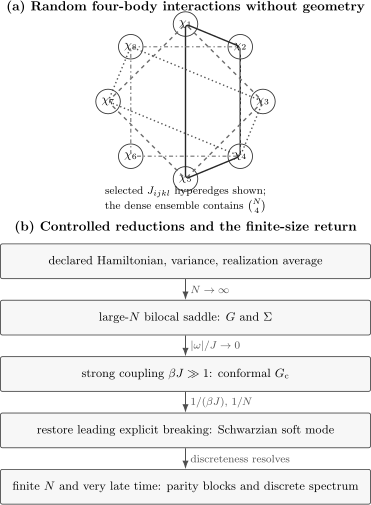
The baseline SYK model is a zero-dimensional random hypergraph: each coupling joins $q$ distinct Majorana modes, with no spatial distance attached. Controlled reductions require declared limits. The bilocal saddle follows after the ensemble and large-$N$ limit; the conformal form requires $\beta J\gg1$; restoring the leading explicit breaking produces the Schwarzian soft mode. Finite-$N$ spectra and very late times must return to the parity-resolved matrix problem.

Thermodynamic Fingerprints

Evaluating the Schwarzian action near its thermal saddle gives

$$\ln Z = -\beta E_0 +S_0 + \frac{2\pi^2C}{\beta} + \cdots.$$

Consequently,

$$F(T) = E_0 -S_0T -2\pi^2CT^2 + \cdots,$$

and

$$C_V = 4\pi^2CT + \cdots.$$

Because $C\propto N/J$, the low-temperature heat capacity is extensive and linear in $T$ within the Schwarzian regime.

Residual entropy and its order of limits

The large-$N$ saddle has

$$S_0 = Ns_0(q).$$

For the standard $q=4$ Majorana normalization,

$$s_0(4) \simeq 0.2324.$$

The statement is

$$\lim_{\beta J\to\infty} \lim_{N\to\infty} \frac{S}{N} = s_0(q)>0.$$

At fixed finite $N$, the spectrum is discrete. Taking $T\to0$ first leaves only the finite ground-state degeneracy $g_0$:

$$\lim_{\beta\to\infty} S_N(\beta) = \ln g_0,$$

so

$$\lim_{N\to\infty} \lim_{\beta\to\infty} \frac{S_N}{N} = 0$$

when $g_0$ is not exponentially large. Calling $S_0$ an extensive degeneracy of every finite Hamiltonian reverses the limits.

Four-Point Functions and Scrambling

Leading connected four-point functions are $O(1/N)$ and are obtained by summing ladder diagrams. Their kernel is built from the saddle Green function. Different Euclidean, retarded, and out-of-time-order continuations probe different eigenvalue problems, so one cannot infer an OTOC exponent from an ordinary time-ordered decay without performing the continuation.

A regularized thermal OTOC can be written schematically as

$$\begin{aligned} F(t) &= \frac1N \sum_{i,j} \operatorname{Tr} \Big[ y\chi_i(t)y\chi_j \\ &\quad \times y\chi_i(t)y\chi_j \Big], \\ y^4 &= \frac{e^{-\beta H}}{Z}. \end{aligned}$$

After subtracting or normalizing the disconnected contribution, the large-$N$ strong-coupling result contains a window

$$\delta F(t) \sim \frac1N e^{\lambda_L t}.$$

In the low-temperature limit,

$$\lambda_L = \frac{2\pi}{\beta} \left[ 1 + O\!\left( \frac{1}{\beta J} \right) \right].$$

Restoring units,

$$\lambda_L \longrightarrow \frac{2\pi k_{\mathrm B}T}{\hbar}$$

at leading strong coupling. This saturates the Maldacena–Shenker–Stanford bound under its analyticity and factorization assumptions.

The exponential cannot continue indefinitely. It becomes order one near

$$t_\ast \sim \lambda_L^{-1}\ln N,$$

up to convention- and temperature-dependent constants. The result refers to an intermediate large-$N$ window after microscopic transients and before saturation. At finite $N$, an exact correlator is bounded and quasiperiodic.

Because the baseline model has no space, it has no geometric butterfly velocity. Operator size, meaning the number of Majoranas in an operator string, replaces spatial radius as a useful growth coordinate. The general definitions, contour choices, and inference cautions belong to Scrambling and OTOCs Preview.

Finite-N Spectra and the Mod-8 Pattern

For $q=4$ and even $N$, antiunitary structure depends on $N\bmod8$. After resolving fermion parity, the bulk random-matrix class follows this cycle:

$N\bmod8$	class inside one parity block	antiunitary action	forced structure
$0$	GOE, class AI	preserves parity and squares to $+1$	no generic Kramers degeneracy
$2$	GUE, class A	exchanges the two parity sectors	opposite-parity spectra are paired
$4$	GSE, class AII	preserves parity and squares to $-1$	Kramers pairs within a block
$6$	GUE, class A	exchanges the two parity sectors	opposite-parity spectra are paired

The table is not universal for every $q$, every added symmetry, or complex SYK. In particular, changing $q\bmod4$ changes the antiunitary classification.

What random-matrix agreement means

For dense $q=4$ SYK, numerical and analytic work supports:

• Wigner–Dyson bulk spacing statistics in the appropriate class;
• a correlation hole, ramp, and plateau in suitably averaged spectral form factors;
• a Thouless crossover separating model-specific correlations from later random-matrix behavior;
• a Heisenberg time set by the exponentially small many-body level spacing.

It does not mean that the smooth density of states is a Wigner semicircle, that all energies are universal, or that one short spectrum has enough levels to identify a class. SYK’s global density has its own $q$- and $N$-dependent structure. Random-matrix universality concerns local fluctuations after the smooth density and exact sectors have been handled.

Quantum Chaos Preview gives the canonical audit for level ratios, unfolding, form factors, filtering, and uncertainty.

Scale and Limit Ledger

Regime or scale	Typical condition	Controlled statement	What ends it
microscopic	$t\sim J^{-1}$	full Hamiltonian and ultraviolet Green function	no simplification assumed
large-N saddle	$N\to\infty$ at fixed $\beta J$	closed equations for $G$ and $\Sigma$	$1/N$ fluctuations
conformal	$\beta J\gg1$, frequencies $\ll J$	$\Delta=1/q$ and conformal correlator	derivative term and UV completion
Schwarzian	soft reparametrization sector	leading explicit breaking and low-$T$ thermodynamics	higher irrelevant operators and strong finite-$N$ fluctuations
Lyapunov window	after transients, before $t_\ast$	$\delta F\sim N^{-1}e^{\lambda_Lt}$	OTOC becomes order one
spectral RMT	after a model-dependent Thouless scale	symmetry-class fluctuation universality	spectral edges, short times, unresolved sectors
Heisenberg	$t_{\mathrm H}\sim2\pi/\Delta E$	discreteness and plateau	recurrences and sample specificity

No single ordering of every intermediate scale holds for arbitrary joint scalings of $N$, $q$, and $\beta J$. A calculation should state which parameters are held fixed.

Solution-Status Ledger

Question	Status	Main route
finite realization spectrum	exact numerically, not closed-form generically	parity-resolved exact diagonalization or Krylov methods
ensemble second moments	exact combinatorics	Clifford trace orthogonality
leading large-N two-point function	controlled implicit solution	Schwinger–Dyson equations
infrared two-point function	analytic leading scaling form	conformal saddle
leading connected four-point function	controlled at large N	ladder-kernel inversion
leading soft mode	controlled low-energy effective theory	Schwarzian action
finite-N spectral fluctuations	class and regime dependent	symmetry analysis, sampling, and RMT
one-realization holographic interpretation	not established as a general theorem	active and conjectural research

The phrase “the SYK model is exactly solvable” therefore needs a qualifier. The disorder-averaged large-$N$ saddle is tractable and many infrared quantities are analytic. A generic finite realization is still an exponentially large interacting matrix problem.

Observable–Method Dictionary

Target	Definition must include	Reliable methods
Euclidean $G(\tau)$	Majorana sign and normalization	Schwinger–Dyson iteration, Monte Carlo, ED
spectral density	analytic-continuation convention and broadening	real-frequency saddle methods, maximum entropy with caution, Krylov/ED
free energy and entropy	quenched or annealed average; order of limits	saddle action, thermodynamic integration, ED
OTOC	contour regularization and disconnected subtraction	ladder kernel, real-time Krylov, protocol simulation
level statistics	parity and antiunitary class; energy window	symmetry-resolved ED and disorder sampling
spectral form factor	connected/full, filtering, normalization, averaging	ED, stochastic trace methods
sample fluctuations	distribution and number of realizations	replica or supersymmetric methods, direct sampling

Important Limits and Variants

q=2: random quadratic Majoranas

For $q=2$,

$$H_2 = i\sum_{i<j} J_{ij}\chi_i\chi_j.$$

A real orthogonal transformation reduces the antisymmetric coupling matrix to $2\times2$ blocks. The Hamiltonian becomes

$$H_2 = \sum_{a=1}^{N/2} \varepsilon_a \left( d_a^\dagger d_a-\frac12 \right).$$

It is a random free-fermion model. It can have random one-particle levels but lacks the interacting melonic saddle and maximal strong-coupling scrambling of $q\geq4$ SYK. “Random” does not imply “interacting chaotic.”

Complex SYK

Complex fermions with random charge-conserving interactions have a global $U(1)$ charge, a chemical potential, spectral asymmetry, and an additional phase mode. Their Green functions and thermodynamics require a filling or charge sector. Majorana formulas cannot be transferred unchanged.

Mixed q=2 and q=4

Adding a quadratic term introduces a relevant competition between free and interacting behavior:

$$H = H_4 +\kappa H_2.$$

The crossover depends on $\kappa$, temperature, and order of limits. It is not obtained by simply replacing $J$ in the pure-$q$ saddle.

Sparse ensembles

Dense $q$-body SYK contains $\binom Nq$ random terms. Sparse variants retain only a subset, often with a connectivity scaling chosen as $N$ grows. Their symmetry accidents, chaos threshold, and coupling normalization require a separate declaration. The twelve-term matrix below is a benchmark fixture, not a claim about a sparse large-$N$ phase.

Tensor and disorder-free relatives

Tensor models can reproduce melonic large-$N$ counting without quenched disorder. They have different microscopic symmetries and index structures. Sharing leading diagrams does not make their finite spectra identical to SYK.

Chains, lattices, and coupled dots

Spatial arrays of SYK-like units can support diffusion, transport, and a butterfly velocity. Those properties arise from the added intersite couplings and geometry. They are not observables of the zero-dimensional baseline Hamiltonian.

Deterministic N=8 Matrix Benchmark

This checkpoint tests operator normalization, signs, parity, basis ordering, and diagonalization. It intentionally does not test disorder-averaged chaos.

Jordan–Wigner representation

Use four qubits and

$$\begin{aligned} \chi_{2a-1} &= \frac{1}{\sqrt2} \left( \prod_{b<a}Z_b \right) X_a, \\ \chi_{2a} &= \frac{1}{\sqrt2} \left( \prod_{b<a}Z_b \right) Y_a, \\ a &= 1,\ldots,4. \end{aligned}$$

Then

$$P = Z_1Z_2Z_3Z_4.$$

Set $q=4$ and write

$$H_{\mathrm{bench}} = -J \sum_I j_I\chi_I.$$

Only the following twelve dimensionless couplings are nonzero:

$I$	$j_I$	$I$	$j_I$
$1234$	$1.00$	$1235$	$-0.73$
$1246$	$0.41$	$1257$	$0.88$
$1268$	$-0.57$	$1347$	$0.69$
$1358$	$0.52$	$1456$	$-0.64$
$1467$	$0.37$	$1568$	$-0.46$
$2348$	$-0.31$	$2356$	$0.59$

Here $\chi_{1234}$ means $\chi_1\chi_2\chi_3\chi_4$. Of the $66$ unordered pairs of listed monomials, $27$ do not commute, so this is not a disguised sum of mutually commuting terms.

Exact invariants

The $16\times16$ matrix obeys

$$\begin{aligned} H_{\mathrm{bench}}^\dagger &= H_{\mathrm{bench}}, \\ [H_{\mathrm{bench}},P] &= 0, \\ \operatorname{Tr}H_{\mathrm{bench}} &= 0. \end{aligned}$$

Trace orthogonality gives

$$\begin{aligned} \frac{\operatorname{Tr}H_{\mathrm{bench}}^2}{J^2} &= \sum_I j_I^2 \\ &= 4.7491. \end{aligned}$$

Parity-resolved eigenvalues

The eigenvalues in units of $J$, sorted within each parity block, are:

index	$P=+1$	$P=-1$
1	$-0.7999661940$	$-1.1096893852$
2	$-0.6045478844$	$-0.4552562301$
3	$-0.3613504879$	$-0.2324994716$
4	$-0.0104565917$	$0.0108652721$
5	$0.0830759460$	$0.2257337478$
6	$0.1469752766$	$0.4244626075$
7	$0.6880946030$	$0.5186979869$
8	$0.8581753324$	$0.6176854727$

A reproduction should satisfy

$$\max_k \left| E_k^{\mathrm{num}} -E_k^{\mathrm{tab}} \right| < 5\times10^{-10}J$$

and

$$\left| \frac{\operatorname{Tr}H^2}{J^2} -4.7491 \right| < 10^{-12}.$$

The ground state lies in the $P=-1$ block. These numbers depend on the stated Jordan–Wigner ordering and the $q=4$ minus sign, while the full spectrum is invariant under a consistent basis change.

Numerical Workflow

A finite-$N$ study should record:

1. $N$, $q$, Majorana normalization, and coupling variance;
2. the random-number generator and seed for every realization;
3. dense versus sparse term selection;
4. fermion-parity and antiunitary sector construction;
5. matrix basis and bit ordering;
6. energy window, edge cuts, and unfolding or gap-ratio choice;
7. number of disorder samples and uncertainty bars;
8. whether observables are averaged before or after nonlinear operations;
9. time-step, Krylov tolerance, and trace-estimation error for dynamics;
10. checks against trace moments and exact small-$N$ matrices.

For level statistics, diagonalizing the full matrix and then deleting obvious degeneracies is not equivalent to constructing irreducible blocks first. For OTOCs, averaging an exponentially growing fit parameter over samples is not equivalent to fitting the averaged correlator.

Common Mistakes

Treating SYK as one Hamiltonian

SYK names an ensemble family. $N$, $q$, operator normalization, variance, charge structure, sparsity, and averaging prescription are part of the definition.

Calling N the particle number

$N$ counts Majorana modes. The Hilbert space contains all occupations of $N/2$ complex modes unless an additional charge constraint is imposed.

Using the conformal propagator in the ultraviolet

Dropping the derivative term removes the canonical short-time condition. The conformal expression is an infrared asymptotic form, not a globally normalized Green function.

Reversing the entropy limits

The extensive residual entropy belongs to $N\to\infty$ before $T\to0$. It is not an exponentially degenerate ground space of every finite sample.

Calling every q random model chaotic

$q=2$ is quadratic. Sparse models can develop extra symmetries. A random coupling list does not replace a symmetry-resolved diagnostic.

Assigning one random-matrix class to all N

For Majorana $q=4$, the class cycles with $N\bmod8$. Complex SYK and other $q\bmod4$ values have different classifications.

Extending Lyapunov growth forever

The $N^{-1}e^{\lambda_Lt}$ term belongs to an intermediate window. Finite-dimensional correlators saturate and eventually resolve discreteness.

Importing spatial language

The single-dot model has no distance or butterfly velocity. Those require an added geometry.

Equating a shared Schwarzian with a complete duality

Matching low-energy effective actions is strong structural evidence for a common sector. It does not identify every microscopic observable or every finite realization with a unique gravity theory.

Exercises

1. Hermiticity and ensemble scaling

Show that $i^{q/2}\chi_{i_1}\cdots\chi_{i_q}$ is Hermitian for even $q$. Then derive the ensemble-averaged second moment

$$\frac{1}{2^{N/2}} \overline{\operatorname{Tr}H_q^2}.$$

Solution

Reversing a product of $q$ distinct Majoranas requires $q(q-1)/2$ exchanges:

$$\left( \chi_{i_1}\cdots\chi_{i_q} \right)^\dagger = (-1)^{q(q-1)/2} \chi_{i_1}\cdots\chi_{i_q}.$$

For even $q$,

$$\left(-i\right)^{q/2} (-1)^{q(q-1)/2} = i^{q/2},$$

so the phased monomial is Hermitian.

Distinct Clifford monomials are trace orthogonal, and each ordered monomial has normalized squared trace $2^{-q}$. Therefore

$$\begin{aligned} \frac{1}{2^{N/2}} \overline{\operatorname{Tr}H_q^2} &= \binom Nq \frac{(q-1)!J^2}{N^{q-1}} \frac1{2^q} \\ &= \frac{NJ^2}{q\,2^q} \prod_{r=0}^{q-1} \left(1-\frac rN\right). \end{aligned}$$

It scales as $N$ at fixed $q$.

2. Why q=2 is free

Let $J_{ij}=-J_{ji}$ and write

$$H_2 = \frac{i}{2} \sum_{i,j} J_{ij}\chi_i\chi_j.$$

Show that an orthogonal Majorana transformation reduces $H_2$ to independent fermionic levels. Why does random one-particle level repulsion not establish interacting many-body scrambling?

Solution

Every real antisymmetric matrix can be brought by an orthogonal matrix $O$ to canonical blocks,

$$OJO^{\mathsf T} = \bigoplus_a \begin{pmatrix} 0 & \varepsilon_a\\ -\varepsilon_a & 0 \end{pmatrix}.$$

With transformed Majoranas $\widetilde\chi=O\chi$ and

$$d_a = \frac{ \widetilde\chi_{2a-1} +i\widetilde\chi_{2a} }{\sqrt2},$$

one obtains

$$H_2 = \sum_a \varepsilon_a \left( d_a^\dagger d_a-\frac12 \right).$$

The many-body energies are sums of independent one-particle occupations. Randomness can produce nontrivial statistics for the $\varepsilon_a$, but there is no interaction-induced ladder kernel or growth from one fermion string into progressively larger strings. Spectral randomness and interacting scrambling are different claims.

3. Determine the infrared dimension

Assume

$$G(\tau) \sim \frac{\operatorname{sgn}\tau}{|\tau|^{2\Delta}}, \qquad \Sigma(\tau) \sim G(\tau)^{q-1}.$$

Use the infrared convolution equation $G\ast\Sigma=-\delta$ to determine $\Delta$.

Solution

The product of scaling dimensions in the convolution behaves as

$$G(\tau_1-\tau) \Sigma(\tau-\tau_2) \sim |\tau|^{-2q\Delta}.$$

One time integration changes the scaling power by $+1$, so the convolution has dimension

$$|\tau|^{1-2q\Delta}.$$

It must match $\delta(\tau)$, which scales as $|\tau|^{-1}$. Hence

$$1-2q\Delta = -1,$$

and therefore

$$\Delta = \frac1q.$$

4. Audit the residual entropy

Suppose a sequence of finite systems has a nondegenerate ground state but approaches the large-$N$ saddle with entropy density $s_0>0$. Evaluate the two iterated limits of $S_N(\beta)/N$ and explain why there is no contradiction.

Solution

At every fixed $N$, taking $\beta\to\infty$ first gives

$$S_N \longrightarrow \ln g_0 = 0$$

for a nondegenerate ground state. Thus

$$\lim_{N\to\infty} \lim_{\beta\to\infty} \frac{S_N}{N} = 0.$$

At fixed large but finite $\beta J$, taking $N\to\infty$ first produces an exponentially dense low-energy spectrum and the saddle entropy. Taking $\beta J\to\infty$ afterward gives

$$\lim_{\beta J\to\infty} \lim_{N\to\infty} \frac{S_N}{N} = s_0.$$

The limits inspect different spectral resolutions. The first resolves the finite-$N$ ground state; the second retains an exponentially dense large-$N$ near-ground-state band.

5. Resolve the mod-8 class

For Majorana $q=4$, identify the parity-resolved random-matrix expectations for $N=12$ and $N=14$. State which degeneracies must be handled before computing gap ratios.

Solution

For $N=12$,

$$N\bmod8 = 4.$$

The antiunitary symmetry preserves parity and squares to $-1$. Each parity block is in the GSE class and contains Kramers pairs. One must retain one representative from each exact Kramers pair, using the appropriate symplectic convention, before forming ordinary consecutive gaps.

For $N=14$,

$$N\bmod8 = 6.$$

Each individual parity block is in the GUE class, while the antiunitary symmetry exchanges the two parity sectors. Their spectra are paired across parity. Gap statistics should be computed in one parity block at a time; pooling the paired blocks duplicates every level.

6. Reproduce the finite benchmark

Use the twelve listed $N=8$ couplings. Without diagonalizing, derive $\operatorname{Tr}H^2/J^2$. Then use the tabulated spectra to identify the ground-state parity and check the full trace.

Solution

For $N=8$, the Hilbert-space dimension is $16$. Every four-Majorana monomial squares to $1/16$, and distinct monomials are trace orthogonal. Thus

$$\frac{\operatorname{Tr}H^2}{J^2} = \sum_I j_I^2.$$

Substitution gives

$$\sum_Ij_I^2 = 4.7491.$$

The lowest listed value is

$$E_0 = -1.1096893852J$$

in the $P=-1$ block.

Adding all sixteen tabulated eigenvalues gives zero within rounding, in agreement with

$$\operatorname{Tr}H = 0.$$

This validates the basis and sign convention but does not establish a disorder-averaged spacing law: the fixture is one deliberately sparse deterministic matrix.

Key Takeaways

• SYK is an ensemble family, not a parameter-free Hamiltonian.
• The Majorana normalization and coupling variance must be stated together.
• Its solvability is the controlled disorder-averaged large-$N$ saddle, not a generic closed-form finite spectrum.
• The conformal solution is infrared and requires the derivative term for ultraviolet completion.
• The Schwarzian action controls a soft reparametrization sector and low-temperature corrections.
• Maximal Lyapunov growth occurs in a specified strong-coupling, large-$N$ time window.
• Finite-$N$ spectral statistics require parity resolution and the $N\bmod8$ class.
• Residual entropy, late-time plateaus, and holographic claims are all sensitive to order of limits.

Cross-Links

• Model Encyclopedia for model-family comparisons and dossier conventions;
• Large-N and Saddle-Point Methods Preview for the general asymptotic machinery;
• Scrambling and OTOCs Preview for contours, bounds, velocities, and protocols;
• Quantum Chaos Preview for spectral diagnostics and random-matrix inference;
• Euclidean and Imaginary-Time Path Integrals for thermal functional integrals;
• Thermal Density Operators for canonical expectations;
• Time-Dependent Correlations for spectral representations and analytic continuation;
• Thermodynamic Limit for noncommuting limits and extensivity;
• Scaling of Hilbert Space for finite-basis growth;
• Benchmark Problems for broader numerical validation practice.

References

1. S. Sachdev and J. Ye, “Gapless Spin-Fluid Ground State in a Random Quantum Heisenberg Magnet”, Physical Review Letters 70, 3339–3342 (1993).
2. A. Kitaev, “A Simple Model of Quantum Holography” and part II, KITP talks (2015).
3. J. Polchinski and V. Rosenhaus, “The Spectrum in the Sachdev–Ye–Kitaev Model”, Journal of High Energy Physics 2016, 1 (2016).
4. J. Maldacena and D. Stanford, “Remarks on the Sachdev–Ye–Kitaev Model”, Physical Review D 94, 106002 (2016).
5. J. Maldacena, S. H. Shenker, and D. Stanford, “A Bound on Chaos”, Journal of High Energy Physics 2016, 106 (2016).
6. A. M. García-García and J. J. M. Verbaarschot, “Spectral and Thermodynamic Properties of the Sachdev–Ye–Kitaev Model”, Physical Review D 94, 126010 (2016).
7. Y.-Z. You, A. W. W. Ludwig, and C. Xu, “Sachdev–Ye–Kitaev Model and Thermalization on the Boundary of Many-Body Localized Fermionic Symmetry-Protected Topological States”, Physical Review B 95, 115150 (2017).
8. J. S. Cotler et al., “Black Holes and Random Matrices”, Journal of High Energy Physics 2017, 118 (2017), with erratum.
9. D. Stanford and E. Witten, “Fermionic Localization of the Schwarzian Theory”, Journal of High Energy Physics 2017, 8 (2017).
10. A. Kitaev and S. J. Suh, “The Soft Mode in the Sachdev–Ye–Kitaev Model and Its Gravity Dual”, Journal of High Energy Physics 2018, 183 (2018).
11. D. A. Roberts, D. Stanford, and A. Streicher, “Operator Growth in the SYK Model”, Journal of High Energy Physics 2018, 122 (2018).
12. V. Rosenhaus, “An Introduction to the SYK Model”, Journal of Physics A: Mathematical and Theoretical 52, 323001 (2019).
13. F. Sun and J. Ye, “Periodic Table of SYK and Supersymmetric SYK”, Physical Review Letters 124, 244101 (2020).
14. B. Kobrin et al., “Many-Body Chaos in the Sachdev–Ye–Kitaev Model”, Physical Review Letters 126, 030602 (2021).
15. D. Chowdhury, A. Georges, O. Parcollet, and S. Sachdev, “Sachdev–Ye–Kitaev Models and Beyond: Window into Non-Fermi Liquids”, Reviews of Modern Physics 94, 035004 (2022).

Further Reading

• J. Maldacena, D. Stanford, and Z. Yang, “Conformal Symmetry and Its Breaking in Two-Dimensional Nearly Anti-de Sitter Space”, Progress of Theoretical and Experimental Physics 2016, 12C104 (2016).
• Y. Gu, A. Kitaev, S. Sachdev, and G. Tarnopolsky, “Notes on the Complex Sachdev–Ye–Kitaev Model”, Journal of High Energy Physics 2020, 157 (2020).
• A. M. García-García, Y. Jia, D. Rosa, and J. J. M. Verbaarschot, “Sparse Sachdev–Ye–Kitaev Model, Quantum Chaos, and Gravity Duals”, Physical Review D 103, 106002 (2021).