Bose–Hubbard Dimer

One-Sentence Description

The Bose–Hubbard dimer is the two-mode bosonic model in which tunneling competes with onsite interactions; every fixed-particle-number sector is finite, and the $N=2$ sector gives a complete analytic laboratory for bosonic enhancement, number squeezing, fragmentation, pair formation, and coherent tunneling.

This dossier owns the finite two-mode problem: its basis, matrix elements, spin representation, exact low-particle spectra, observables, dynamics, asymptotic limits, and reproducible checks. The Bose–Hubbard Model article owns the general lattice model, atomic-limit Mott physics, optical-lattice reduction, and thermodynamic phase boundary. MB-B005 remains the stable numerical contract.

Baseline Model Record

Unless a variant is stated explicitly, this page uses:

Field	Baseline choice
modes	two bosonic modes, labeled $1$ and $2$
local occupation	$n_i=0,1,2,\ldots$
primary sector	fixed total particle number $N$
bond list	one undirected bond $\{1,2\}$
hopping	real $J>0$, with one-particle matrix element $-J$
interaction	onsite $U\in\mathbb R$
bias	absent
chemical potential	absent because one fixed-$N$ sector is diagonalized
exchange symmetry	exact interchange $1\leftrightarrow2$
benchmark sector	$N=2$
benchmark point	$J=1$, $U=2$

The dimer has one physical link. Writing a two-site periodic nearest-neighbor sum and then adding its Hermitian conjugate can count that link twice. A calculation is reproducible only after the bond convention and the meaning of $J$ are stated.

Bosonic Hilbert Space

The mode operators satisfy

$$\begin{aligned} [b_i,b_j^\dagger] &= \delta_{ij}I, \\ [b_i,b_j] &= [b_i^\dagger,b_j^\dagger] =0, \end{aligned}$$

with number operators $n_i=b_i^\dagger b_i$. Their action on a normalized occupation state is

$$\begin{aligned} b_1\lvert n_1,n_2\rangle &= \sqrt{n_1}\, \lvert n_1-1,n_2\rangle, \\ b_1^\dagger\lvert n_1,n_2\rangle &= \sqrt{n_1+1}\, \lvert n_1+1,n_2\rangle, \end{aligned}$$

and similarly for mode $2$.

The unrestricted two-mode Fock space is infinite dimensional. The Hamiltonian conserves

$$\widehat N=n_1+n_2,$$

so a fixed-$N$ basis is

$$\mathcal B_N = \bigl\{ \lvert n,N-n\rangle: n=0,1,\ldots,N \bigr\}.$$

Its dimension is

$$\dim\mathcal H_N=N+1.$$

No additional onsite cutoff is needed in this sector: number conservation already implies $0\le n_i\le N$. A cutoff smaller than $N$ changes the model by deleting valid states.

Hamiltonian and Conventions

The symmetric dimer Hamiltonian is

$$\begin{aligned} H ={}& -J \left( b_1^\dagger b_2 + b_2^\dagger b_1 \right) \\ &+ \frac{U}{2} \left[ n_1(n_1-1) + n_2(n_2-1) \right]. \end{aligned}$$

The hopping term delocalizes particles. Repulsive $U>0$ suppresses occupation imbalance and onsite pairs, while attractive $U<0$ favors clustering. The interaction counts unordered pairs: a mode with $n$ bosons contributes $Un(n-1)/2$.

At fixed $N$, adding $-\mu\widehat N$ shifts every eigenvalue by $-\mu N$ without changing eigenvectors or level spacings. The chemical potential matters only when sectors with different $N$ compete.

Occupation-basis matrix

Write

$$\lvert n\rangle_N \equiv \lvert n,N-n\rangle.$$

The diagonal element is

$$\begin{aligned} d_n &= \frac{U}{2} \left[ n(n-1) + (N-n)(N-n-1) \right] \\ &= U \left[ \left(n-\frac N2\right)^2 + \frac{N(N-2)}{4} \right]. \end{aligned}$$

The only nonzero off-diagonal element connecting neighboring occupations is

$${}_N\langle n+1\rvert H\lvert n\rangle_N = -J\sqrt{(n+1)(N-n)}.$$

The factor under the square root is the bosonic enhancement. Replacing it by a constant $J$ turns the calculation into a different tight-binding problem in occupation space.

If

$$\lvert\psi\rangle = \sum_{n=0}^{N}c_n\lvert n\rangle_N,$$

then the eigenvalue equation is the finite recurrence

$$\begin{aligned} E c_n ={}& d_n c_n - J\sqrt{n(N-n+1)}\,c_{n-1} \\ &- J\sqrt{(n+1)(N-n)}\,c_{n+1}, \end{aligned}$$

with $c_{-1}=c_{N+1}=0$. Thus every fixed-$N$ problem is a real symmetric tridiagonal matrix of order $N+1$.

Schwinger-Spin Representation

Define

$$\begin{aligned} S_x &= \frac12 \left( b_1^\dagger b_2+b_2^\dagger b_1 \right), \\ S_y &= \frac{1}{2i} \left( b_1^\dagger b_2-b_2^\dagger b_1 \right), \\ S_z &= \frac12(n_1-n_2). \end{aligned}$$

These operators obey $[S_a,S_b]=i\epsilon_{abc}S_c$. In the fixed-$N$ sector,

$$S=\frac N2, \qquad \mathbf S^2=S(S+1)I.$$

The Hamiltonian becomes

$$H = -2J S_x + U S_z^2 + \frac{U N(N-2)}{4}I.$$

The dimer is therefore a single spin $S=N/2$ in a transverse field with quadratic, one-axis anisotropy. The final term is constant at fixed $N$; dropping it is harmless for eigenvectors and gaps but changes absolute energies. Any comparison must say whether that offset was retained.

The occupation state $\lvert n,N-n\rangle$ corresponds to the spin state

$$\lvert S,m\rangle, \qquad m=n-\frac N2.$$

This map is exact. It is not a large-$N$ or mean-field approximation.

Symmetries and Conserved Quantities

Number conservation

The global phase symmetry

$$b_i\longmapsto e^{i\alpha}b_i$$

implies

$$[H,\widehat N]=0.$$

It is the reason the infinite Fock space decomposes into finite blocks.

Mode exchange

Let $P$ interchange the two modes:

$$P\lvert n,N-n\rangle = \lvert N-n,n\rangle.$$

For the unbiased dimer,

$$[H,P]=0, \qquad P^2=I.$$

Eigenstates may be assigned reflection parity $p=\pm1$. In spin language, the interchange sends $S_z\mapsto-S_z$ and leaves $S_x$ unchanged. A bias proportional to $n_1-n_2$ breaks this symmetry.

Reality and time reversal

In the declared occupation basis, $H$ is real symmetric. Complex conjugation is therefore a time-reversal symmetry for this spinless two-mode model. A tunneling phase can be removed on one isolated link by rephasing a mode; unlike a loop, a single dimer carries no gauge-invariant flux.

Ground-state parity

For $J>0$, all off-diagonal entries of the irreducible fixed-$N$ matrix are negative. The Perron–Frobenius argument permits a nondegenerate ground state with strictly positive occupation-basis coefficients. Since mode exchange preserves positivity and commutes with $H$, that ground state is even under $P$ for every finite $N$ and finite $U$.

This statement matters in the attractive regime: the finite-system ground state is an even cat-like superposition, not a state localized permanently in one well. An arbitrarily small bias can nevertheless select one side once it exceeds the exponentially small parity splitting.

Exact Solution Status

Object	Status	Qualification
fixed-$N$ Hilbert space	exact	dimension $N+1$
matrix representation	exact	real symmetric tridiagonal recurrence
$N=0,1,2$ spectrum	elementary closed form	all eigenvectors and observables are analytic
arbitrary finite $N$	finite exact diagonalization	complete after the basis and arithmetic precision are declared
Bethe-ansatz description	available	algebraic and differential-equation formulations exist, but roots still require solving coupled algebraic equations
large-$N$ phase-space dynamics	controlled semiclassical limit	finite-$N$ tunneling, revivals, and parity restoration are quantum corrections
thermodynamic phase transition	not defined for one fixed dimer	sharp transitions require an additional scaling limit

Calling the dimer “exactly solved” is useful only with an object attached. The $(N+1)\times(N+1)$ matrix is exact for every finite $N$, while a compact formula in elementary functions for every eigenvalue is unavailable at generic $N$.

Elementary Sectors

Vacuum sector

For $N=0$, the only state is $\lvert0,0\rangle$ and $E=0$.

One boson

In the basis $\{\lvert1,0\rangle,\lvert0,1\rangle\}$,

$$H_{N=1} = \begin{pmatrix} 0 & -J\\ -J & 0 \end{pmatrix}.$$

The bonding and antibonding states are

$$\lvert\pm\rangle = \frac{ \lvert1,0\rangle \pm \lvert0,1\rangle }{\sqrt2},$$

with energies $E_+=-J$ and $E_-=+J$, where the subscript here denotes exchange parity. The interaction is invisible because one particle cannot form an onsite pair.

Exact Two-Boson Problem

For $N=2$, use the ordered basis

$$\mathcal B_2 = \bigl\{ \lvert2,0\rangle, \lvert1,1\rangle, \lvert0,2\rangle \bigr\}.$$

The Hamiltonian is

$$H_{N=2} = \begin{pmatrix} U & -\sqrt2J & 0\\ -\sqrt2J & 0 & -\sqrt2J\\ 0 & -\sqrt2J & U \end{pmatrix}.$$

The matrix element $-\sqrt2J$ follows, for example, from

$$\begin{aligned} \langle1,1\rvert b_2^\dagger b_1 \lvert2,0\rangle &= \sqrt2, \\ \langle1,1\rvert H\lvert2,0\rangle &= -\sqrt2J. \end{aligned}$$

Parity reduction

Introduce even and odd pair states

$$\begin{aligned} \lvert D_+\rangle &= \frac{ \lvert2,0\rangle+\lvert0,2\rangle }{\sqrt2}, \\ \lvert D_-\rangle &= \frac{ \lvert2,0\rangle-\lvert0,2\rangle }{\sqrt2}. \end{aligned}$$

The odd state is dark to $\lvert1,1\rangle$:

$$H\lvert D_-\rangle = U\lvert D_-\rangle.$$

In the even basis $\{\lvert D_+\rangle,\lvert1,1\rangle\}$,

$$H_{\mathrm{even}} = \begin{pmatrix} U & -2J\\ -2J & 0 \end{pmatrix}.$$

The two paths from $\lvert1,1\rangle$ into the left and right doublon states add coherently, changing the coupling from $\sqrt2J$ to $2J$.

Complete spectrum and eigenstates

Define

$$\Delta = \sqrt{U^2+16J^2}.$$

The three eigenvalues are

$$\begin{aligned} E_- &= \frac{U-\Delta}{2}, \\ E_D &=U, \\ E_+ &= \frac{U+\Delta}{2}. \end{aligned}$$

For $J>0$ their ordering is always

$$E_-<E_D<E_+.$$

Choose $0<\theta<\pi/2$ through

$$\cos(2\theta) = \frac{U}{\Delta}, \qquad \sin(2\theta) = \frac{4J}{\Delta}.$$

Normalized eigenstates are

$$\begin{aligned} \lvert\psi_-\rangle &= \cos\theta\, \lvert1,1\rangle + \sin\theta\, \lvert D_+\rangle, \\ \lvert\psi_D\rangle &= \lvert D_-\rangle, \\ \lvert\psi_+\rangle &= \cos\theta\, \lvert D_+\rangle - \sin\theta\, \lvert1,1\rangle. \end{aligned}$$

Both mixed levels have even parity. Their avoided crossing has minimum separation $4J$ at $U=0$. The odd level crosses neither even level because its energy remains between them.

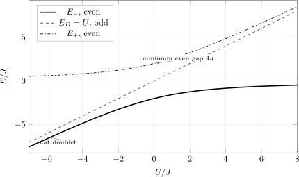
Exact $N=2$ spectrum in units of $J$. The even levels $E_-$ and $E_+$ undergo an avoided crossing, while the odd pair state has $E_D=U$. For large negative $U/J$, $E_-$ and $E_D$ form the nearly degenerate cat-state doublet.

Exact Ground-State Observables for N = 2

Onsite pairs

Define the total onsite-pair operator

$$D_B = \frac12 \sum_{i=1}^{2} n_i(n_i-1).$$

It has eigenvalue $1$ on $\lvert D_\pm\rangle$ and $0$ on $\lvert1,1\rangle$. Therefore

$$\begin{aligned} \langle D_B\rangle_0 &= \sin^2\theta \\ &= \frac12 \left( 1- \frac{U}{\Delta} \right). \end{aligned}$$

The same result follows from Feynman–Hellmann:

$$\langle D_B\rangle_0 = \frac{\partial E_-}{\partial U}.$$

For strong repulsion this probability vanishes as $4J^2/U^2$. For strong attraction it tends to $1$.

Intermode coherence

Let

$$T = b_1^\dagger b_2+b_2^\dagger b_1.$$

Since $\partial H/\partial J=-T$,

$$\langle T\rangle_0 = -\frac{\partial E_-}{\partial J} = \frac{8J}{\Delta}.$$

The coherence per particle is

$$\mathcal C = \frac{\langle T\rangle_0}{N} = \frac{4J}{\Delta}$$

for $N=2$. It equals $1$ at $U=0$ and tends to zero in both strong-interaction limits.

Imbalance fluctuations

Define the population imbalance

$$I=n_1-n_2, \qquad z=\frac{I}{N}.$$

Exchange symmetry gives $\langle I\rangle_0=0$. For two particles,

$$\begin{aligned} \langle I^2\rangle_0 &= 4\sin^2\theta = 2 \left( 1- \frac{U}{\Delta} \right), \\ \langle z^2\rangle_0 &= \sin^2\theta. \end{aligned}$$

Each site has mean occupation $1$ and variance

$$\operatorname{Var}(n_1) = \operatorname{Var}(n_2) = \sin^2\theta.$$

Repulsion squeezes number fluctuations, whereas attraction turns them into macroscopic left-versus-right fluctuations.

One-body density matrix and fragmentation

The one-body density matrix is

$$\rho^{(1)}_{ij} = \langle b_i^\dagger b_j\rangle_0 = \begin{pmatrix} 1 & 4J/\Delta\\ 4J/\Delta & 1 \end{pmatrix}.$$

Its natural occupations are

$$\lambda_\pm = 1\pm\frac{4J}{\Delta}, \qquad \lambda_++\lambda_-=2.$$

At $U=0$, $\lambda_+=2$ and both particles occupy the bonding orbital. In either strong-interaction limit the two natural occupations approach $1$ and $1$. That same limiting spectrum has different many-body interpretations: a number-squeezed product $\lvert1,1\rangle$ for repulsion and a cat-like superposition for attraction.

Mode entanglement

Tracing out either mode leaves occupation probabilities

$$p_0=p_2=\frac{\sin^2\theta}{2}, \qquad p_1=\cos^2\theta.$$

The mode entropy is

$$S_{1|2} = -\cos^2\theta\ln(\cos^2\theta) - \sin^2\theta \ln\left(\frac{\sin^2\theta}{2}\right).$$

This is entanglement between the two mode algebras at fixed number. It should not be confused with an entropy obtained by labeling identical particles.

Exact Two-Boson Dynamics

Prepare one boson in each mode:

$$\lvert\psi(0)\rangle = \lvert1,1\rangle.$$

Parity confines the evolution to the even two-level block. The probability of finding both bosons on the same site at time $t$ is

$$\begin{aligned} P_D(t) &= \lvert\langle D_+\rvert\psi(t)\rangle\rvert^2 \\ &= \frac{16J^2}{\Delta^2} \sin^2\left( \frac{\Delta t}{2\hbar} \right). \end{aligned}$$

This is also $\langle D_B(t)\rangle$. At $U=0$, the system oscillates completely between $\lvert1,1\rangle$ and $\lvert D_+\rangle$ with angular frequency $4J/\hbar$. Repulsion or attraction detunes the pair sector, reduces the maximum transfer probability to $16J^2/\Delta^2$, and raises the oscillation frequency to $\Delta/\hbar$.

The exact finite-$N$ dynamics is quasiperiodic in the many-level case. Mean-field Josephson trajectories can describe a large-$N$ envelope, but they do not reproduce finite-$N$ collapse, revival, parity restoration, or tunneling between semiclassical self-trapped regions.

Important Limits at General N

Noninteracting limit

For $U=0$, introduce bonding and antibonding modes

$$a_+ = \frac{b_1+b_2}{\sqrt2}, \qquad a_- = \frac{b_1-b_2}{\sqrt2}.$$

Then

$$H = -J \left( n_+-n_- \right).$$

If $m$ bosons occupy the antibonding mode, the exact energy and parity are

$$E_m = -J(N-2m), \qquad p_m=(-1)^m, \qquad m=0,1,\ldots,N.$$

The ground state is the number-conserving condensate

$$\lvert\mathrm{bond};N\rangle = \frac{(a_+^\dagger)^N}{\sqrt{N!}} \lvert0\rangle,$$

whose site occupations follow a binomial distribution.

Atomic limit

For $J=0$, every occupation state is an eigenstate with energy $d_n$. Repulsive $U>0$ minimizes occupation imbalance:

• if $N$ is even, the unique ground state is $\lvert N/2,N/2\rangle$;
• if $N$ is odd, the two least-imbalanced states are degenerate.

Attractive $U<0$ instead minimizes the energy with the degenerate endpoint states $\lvert N,0\rangle$ and $\lvert0,N\rangle$.

Strong repulsion and the even–odd effect

For even $N$ and $U\gg J>0$, nondegenerate perturbation theory gives

$$\begin{aligned} E_0 ={}& \frac{U N(N-2)}{4} \\ &- \frac{J^2N(N+2)}{2U} + O\left(\frac{J^4}{U^3}\right). \end{aligned}$$

The first correction is second order because one hop leaves the balanced state.

For odd $N$, the two least-imbalanced states couple directly. Their leading even and odd energies are

$$E_{\mathrm{even/odd}} = \frac{U(N-1)^2}{4} \mp \frac{J(N+1)}{2} + O\left(\frac{J^2}{U}\right).$$

Thus odd filling retains a first-order tunneling scale even when $U/J$ is large. The distinction is a finite-dimer parity effect, not a bulk Mott phase transition.

Strong attraction and cat-state splitting

For $U<0$ and $|U|\gg J$, the endpoint states are connected only after all $N$ bosons tunnel. Degenerate perturbation theory yields the leading parity splitting

$$\delta E_{\mathrm{cat}} = \frac{2N J^N} {(N-1)!\,|U|^{N-1}} \left[ 1+O\left(\frac{J^2}{U^2}\right) \right].$$

The even superposition is the finite-system ground state. Because the splitting falls rapidly with $N$ and $|U|/J$, a small bias, loss process, or dephasing perturbation can destroy coherent left–right superposition physics long before it appreciably changes the larger excitation scales.

Hard-core warning

Taking $U/J\to+\infty$ at fixed $N\le2$ suppresses double occupancy. At $N=2$, only $\lvert1,1\rangle$ remains in the strict projected subspace and hopping has no first-order action. This is not the same as replacing the bosonic ladder factors by spin-$1/2$ matrix elements before taking the limit; projection and perturbative elimination must be performed consistently.

Large-N Phase-Space Connection

A number-conserving product state can be written

$$\lvert\alpha,\beta;N\rangle = \frac{ (\alpha b_1^\dagger+\beta b_2^\dagger)^N }{\sqrt{N!}} \lvert0\rangle, \qquad |\alpha|^2+|\beta|^2=1.$$

Define the classical imbalance and relative phase by

$$z=|\alpha|^2-|\beta|^2, \qquad \phi=\arg\beta-\arg\alpha.$$

The variational energy, apart from a constant, is

$$E_{\mathrm{cl}}(z,\phi) = \frac{U N(N-1)}{4}z^2 - JN\sqrt{1-z^2}\cos\phi.$$

After division by $JN$, the interaction control is

$$\Lambda = \frac{U(N-1)}{2J}.$$

Many references replace $N-1$ by $N$ in the large-$N$ limit. That approximation is harmless asymptotically but should not be inserted into the exact $N=2$ formulas. The phase-space separatrix organizes Josephson oscillations and mean-field self-trapping, with the threshold depending on the initial $z$ and $\phi$. A finite quantum dimer has crossovers and long tunneling times rather than permanently disconnected phase-space regions.

Typical Observables

Observable	Definition	What it diagnoses
imbalance	$I=n_1-n_2=2S_z$	left–right localization and symmetry breaking
coherence	$\mathcal C=\langle b_1^\dagger b_2+b_2^\dagger b_1\rangle/N$	bonding-orbital coherence
onsite pairs	$D_B=\frac12\sum_i n_i(n_i-1)$	interaction energy and clustering
number squeezing	$\xi_n^2=4\operatorname{Var}(S_z)/N$	fluctuations relative to a binomial coherent state
one-body density matrix	$\rho^{(1)}_{ij}=\langle b_i^\dagger b_j\rangle$	natural occupations and fragmentation
parity	$\langle P\rangle$	exchange sector and cat-state coherence
mode entropy	$S_{1\vert2}=-\operatorname{Tr}(\rho_1\ln\rho_1)$	entanglement between mode algebras
current from 1 to 2	$I_{1\to2}=\frac{iJ}{\hbar}(b_2^\dagger b_1-b_1^\dagger b_2)$	coherent particle transfer

The continuity equation is

$$\frac{d n_1}{dt} = -I_{1\to2}, \qquad \frac{d n_2}{dt} = I_{1\to2}.$$

Every observable should be reported with its normalization. In particular, $\langle T\rangle$, $\langle T\rangle/N$, the largest natural occupation, and the condensate fraction are related but numerically different quantities.

Minimal Worked Example: Two Bosons at U = 0

At $U=0$, the two-boson ground state is

$$\begin{aligned} \lvert\mathrm{bond};2\rangle &= \frac{(a_+^\dagger)^2}{\sqrt2} \lvert0\rangle \\ &= \frac12 \left( \lvert2,0\rangle + \sqrt2\lvert1,1\rangle + \lvert0,2\rangle \right). \end{aligned}$$

Its energy is $-2J$. The probability distribution is

$$P(2,0)=\frac14, \qquad P(1,1)=\frac12, \qquad P(0,2)=\frac14.$$

Hence

$$\langle D_B\rangle=\frac12, \qquad \mathcal C=1, \qquad \operatorname{Var}(n_1)=\frac12.$$

The appearance of double occupancy does not signal attraction. It is the binomial fluctuation of two independent bosons condensed into a delocalized orbital.

Numerical Benchmark: MB-B005

The canonical contract is MB-B005: Two-Site Bose–Hubbard Model. Use the ordered basis

$$\bigl\{ \lvert2,0\rangle, \lvert1,1\rangle, \lvert0,2\rangle \bigr\}$$

with $J=1$ and $U=2$. Then

$$\begin{aligned} E_- &= 1-\sqrt5 = -1.236067977499790\ldots, \\ E_D &=2, \\ E_+ &= 1+\sqrt5 = 3.236067977499790\ldots. \end{aligned}$$

The reflection parities are respectively even, odd, and even. At this point,

$$\begin{aligned} \langle D_B\rangle_0 &= \frac12 \left( 1-\frac1{\sqrt5} \right) \\ &= 0.276393202250021\ldots, \\ \mathcal C_0 &= \frac{2}{\sqrt5} = 0.894427190999916\ldots. \end{aligned}$$

The normalized ground state can be audited as

$$\begin{aligned} \lvert\psi_0\rangle ={}& \sqrt{ \frac{1+1/\sqrt5}{2} } \lvert1,1\rangle \\ &+ \sqrt{ \frac{1-1/\sqrt5}{2} } \lvert D_+\rangle. \end{aligned}$$

Matrix invariants

Before diagonalization, verify

$$\begin{aligned} \operatorname{Tr}H &=2U, \\ \operatorname{Tr}H^2 &=2U^2+8J^2, \\ \det H &=-4UJ^2. \end{aligned}$$

At the benchmark point these become $4$, $16$, and $-8$. Also verify Hermiticity, the vanishing commutator $[H,P]$, and the number-sector dimension $3$.

Validation sequence

1. Enumerate the fixed-$N=2$ basis rather than imposing an independent local cutoff.
2. Generate $-\sqrt2J$ from ladder-operator actions.
3. Reproduce all three energies and parities.
4. Check $\langle D_B\rangle_0=\partial E_-/\partial U$.
5. Check $\langle T\rangle_0=-\partial E_-/\partial J$.
6. Set $U=0$ and recover $\{-2J,0,2J\}$.

For a dense $3\times3$ double-precision calculation, absolute residuals near $10^{-12}$ are reasonable. A larger tolerance must be justified by the arithmetic or solver. Agreement with eigenvalues alone is insufficient if observables are evaluated in a differently ordered basis.

Reproducibility status

The planned notebook bose_hubbard_dimer_exact.ipynb is indexed in Reproducible Notebooks. Its admission gate is exact agreement with MB-B005, including parity and both Feynman–Hellmann checks.

Variants and Handoffs

Static bias

An asymmetric dimer adds

$$H_\epsilon = \frac{\epsilon}{2}(n_1-n_2) = \epsilon S_z.$$

This breaks exchange parity, produces $\langle I\rangle\ne0$, and can localize an attractive cat doublet when $|\epsilon|N$ exceeds its tiny tunnel splitting.

Pair tunneling and intermode interaction

Extended dimers may contain

$$V n_1n_2, \qquad P \left[ (b_1^\dagger)^2b_2^2 + (b_2^\dagger)^2b_1^2 \right].$$

These terms change the spin anisotropy and selection rules. Their parameters cannot be folded into $U$ and $J$ without an explicit derivation.

Driven and open junctions

Time-dependent $J(t)$ or $\epsilon(t)$ produces driven tunneling, while particle loss and dephasing require an open-system description. The closed Hamiltonian here remains the baseline against which those additions should be measured.

More sites

The Bose–Hubbard Chain dossier owns the one-dimensional many-site specialization. The broader Bose–Hubbard Model article owns general lattices, Mott lobes, and optical-lattice validity.

Common Mistakes

Missing bosonic enhancement

The $N=2$ hopping matrix element is $-\sqrt2J$, not $-J$. The occupation-dependent square root is part of the operator algebra.

Double-counting the single link

There is one undirected bond. A periodic two-site sum can silently produce $-2J(b_1^\dagger b_2+\mathrm{h.c.})$.

Using Un² instead of Un(n − 1)

The onsite interaction counts pairs. The states $\lvert1,0\rangle$ and $\lvert0,1\rangle$ must have zero interaction energy.

Forgetting the fixed-N constant in the spin map

$H=-2JS_x+US_z^2$ differs from the declared Bose–Hubbard Hamiltonian by $UN(N-2)/4$. Gaps agree; absolute energies generally do not.

Treating a finite crossover as a phase transition

A fixed dimer has a finite Hilbert space and analytic avoided crossings for $J>0$. Mean-field bifurcations and large-$N$ scaling limits require their own qualifications.

Reading zero imbalance as absence of clustering

An even cat state has $\langle n_1-n_2\rangle=0$ but a large imbalance variance. First moments alone cannot distinguish a balanced state from a symmetric superposition of imbalanced states.

Calling every two-mode condensate a Bose–Hubbard dimer

The two-mode approximation assumes a controlled truncation to two orbitals with parameters that do not change appreciably as the state evolves. Strong deformation, higher-band population, density-assisted hopping, or appreciable mode overlap can invalidate the minimal Hamiltonian.

Exercises

1. Derive the fixed-number matrix

For arbitrary $N$, derive the diagonal element $d_n$ and the hopping element between $\lvert n,N-n\rangle$ and $\lvert n+1,N-n-1\rangle$. Explain why the matrix is tridiagonal.

Solution

The interaction is diagonal in the occupation basis:

$$d_n = \frac U2 \left[ n(n-1)+(N-n)(N-n-1) \right].$$

The operator $b_1^\dagger b_2$ moves one boson from mode $2$ to mode $1$:

$$b_1^\dagger b_2 \lvert n,N-n\rangle = \sqrt{(n+1)(N-n)} \lvert n+1,N-n-1\rangle.$$

Its Hermitian conjugate moves one boson in the opposite direction. A single hop changes $n$ only by $\pm1$, so no matrix elements occur beyond the first off-diagonals.

2. Recover the spin Hamiltonian

Use $n_1=N/2+S_z$ and $n_2=N/2-S_z$ to derive the Schwinger-spin form, including its constant term.

Solution

The hopping operator is $2S_x$. For the interaction,

$$\begin{aligned} n_1(n_1-1)+n_2(n_2-1) &= n_1^2+n_2^2-N \\ &= 2S_z^2+\frac{N^2}{2}-N. \end{aligned}$$

Multiplication by $U/2$ gives

$$H = -2JS_x +US_z^2 +\frac{UN(N-2)}{4}I.$$

3. Solve the N = 2 parity blocks

Construct $\lvert D_\pm\rangle$, show that $\lvert D_-\rangle$ is an eigenstate, and diagonalize the even block.

Solution

The hopping amplitudes from $\lvert1,1\rangle$ to the two doublon states are equal. They cancel in the odd combination and add in the even combination:

$$H\lvert D_-\rangle =U\lvert D_-\rangle,$$

while

$$H_{\mathrm{even}} = \begin{pmatrix} U&-2J\\ -2J&0 \end{pmatrix}.$$

Its characteristic polynomial is

$$E^2-UE-4J^2=0,$$

so

$$E_\pm = \frac{U\pm\sqrt{U^2+16J^2}}{2}.$$

Together with $E_D=U$, these are all three eigenvalues.

4. Obtain observables without differentiating eigenvectors

Use the ground-state energy to derive $\langle D_B\rangle_0$ and $\langle T\rangle_0$.

Solution

Because

$$\frac{\partial H}{\partial U}=D_B, \qquad \frac{\partial H}{\partial J}=-T,$$

Feynman–Hellmann gives

$$\begin{aligned} \langle D_B\rangle_0 &= \frac{\partial E_-}{\partial U} = \frac12 \left( 1-\frac{U}{\sqrt{U^2+16J^2}} \right), \\ \langle T\rangle_0 &= -\frac{\partial E_-}{\partial J} = \frac{8J}{\sqrt{U^2+16J^2}}. \end{aligned}$$

5. Explain the repulsive even–odd effect

At $J=0$ and $U>0$, identify the ground manifold for even and odd $N$. Show why the leading tunneling correction is second order for even $N$ but first order for odd $N$.

Solution

For even $N$, the unique minimum is $\lvert N/2,N/2\rangle$. One hop leaves this state, so its first-order diagonal correction vanishes. The two neighboring virtual states each lie an energy $U$ higher, yielding

$$\Delta E^{(2)} = -\frac{J^2N(N+2)}{2U}.$$

For odd $N$, the states

$$\left\lvert\frac{N+1}{2},\frac{N-1}{2}\right\rangle, \qquad \left\lvert\frac{N-1}{2},\frac{N+1}{2}\right\rangle$$

are degenerate and differ by one hop. Their off-diagonal matrix element is

$$-J\frac{N+1}{2}.$$

Diagonalizing this two-state manifold produces a first-order even–odd splitting $J(N+1)$.

6. Derive the pair-oscillation probability

Starting from $\lvert1,1\rangle$, derive the probability of occupying either doublon state at time $t$.

Solution

Only the even block participates. Subtracting $U/2$ times the identity gives the two-level Hamiltonian

$$H_{\mathrm{even}}-\frac U2I = \begin{pmatrix} U/2&-2J\\ -2J&-U/2 \end{pmatrix},$$

whose level separation is $\Delta=\sqrt{U^2+16J^2}$. The standard detuned two-level transition probability is therefore

$$P_D(t) = \frac{(2\cdot2J)^2}{\Delta^2} \sin^2\left( \frac{\Delta t}{2\hbar} \right) = \frac{16J^2}{\Delta^2} \sin^2\left( \frac{\Delta t}{2\hbar} \right).$$

Because $D_B$ projects onto the two-boson pair subspace, $P_D(t)=\langle D_B(t)\rangle$.

Cross-Links

• Model Encyclopedia Overview – dossier conventions and exactness labels.
• Bose–Hubbard Model – canonical many-site Hamiltonian, Mott physics, and optical-lattice reduction.
• Bose–Hubbard Chain – one-dimensional soft-core model, hard-core mapping, and BKT regime.
• Occupation-Number Representation – general bosonic basis construction.
• Bosonic Operators in Many-Body Models – ladder factors and truncation audits.
• Benchmark Problems – stable MB-B005 contract.
• Reproducible Notebooks – planned finite-cluster implementation.
• Hubbard Dimer – fermionic two-site comparison.
• Tight-Binding Dimer – one-particle two-state dynamics.
• Bose–Hubbard Model Card – compact reference entry.

References

• G. J. Milburn, J. Corney, E. M. Wright, and D. F. Walls, “Quantum Dynamics of an Atomic Bose–Einstein Condensate in a Double-Well Potential,” Physical Review A 55, 4318–4324 (1997), doi:10.1103/PhysRevA.55.4318.
• D. Jaksch, C. Bruder, J. I. Cirac, C. W. Gardiner, and P. Zoller, “Cold Bosonic Atoms in Optical Lattices,” Physical Review Letters 81, 3108–3111 (1998), doi:10.1103/PhysRevLett.81.3108.
• S. Raghavan, A. Smerzi, S. Fantoni, and S. R. Shenoy, “Coherent Oscillations between Two Weakly Coupled Bose–Einstein Condensates: Josephson Effects, $\pi$ Oscillations, and Macroscopic Quantum Self-Trapping,” Physical Review A 59, 620–633 (1999), doi:10.1103/PhysRevA.59.620.
• M. Albiez, R. Gati, J. Fölling, S. Hunsmann, M. Cristiani, and M. K. Oberthaler, “Direct Observation of Tunneling and Nonlinear Self-Trapping in a Single Bosonic Josephson Junction,” Physical Review Letters 95, 010402 (2005), doi:10.1103/PhysRevLett.95.010402.
• J. Links and K. E. Hibberd, “Bethe Ansatz Solutions of the Bose–Hubbard Dimer,” SIGMA 2, 095 (2006), doi:10.3842/SIGMA.2006.095.
• R. Gati and M. K. Oberthaler, “A Bosonic Josephson Junction,” Journal of Physics B: Atomic, Molecular and Optical Physics 40, R61–R89 (2007), doi:10.1088/0953-4075/40/10/R01.
• I. Bloch, J. Dalibard, and W. Zwerger, “Many-Body Physics with Ultracold Gases,” Reviews of Modern Physics 80, 885–964 (2008), doi:10.1103/RevModPhys.80.885.