Bose–Hubbard Chain

One-Sentence Description

The Bose–Hubbard chain is the one-dimensional lattice-boson model in which nearest-neighbor tunneling competes with onsite interaction, producing an exactly tractable free limit, an exactly mappable hard-core limit, a generic gapless Luttinger liquid, and interaction-driven Mott insulators at commensurate filling.

This dossier fixes the one-dimensional model, its boundary and momentum conventions, finite-sector construction, exact limits, hard-core map, strong-coupling excitations, infrared diagnostics, and a reproducible finite-chain check. The Bose–Hubbard Model article owns the general lattice Hamiltonian, optical-lattice reduction, atomic intervals, and single-site mean-field boundary. Luttinger Liquid Preview owns the general compact-boson formalism and operator dictionary.

Baseline Model Record

Unless a different choice is stated, this page uses:

Field	Baseline choice
geometry	uniform one-dimensional chain with $L\ge3$ sites
lattice spacing	$a$
local modes	one soft-core bosonic mode per site
hopping	real nearest-neighbor $J>0$
interaction	onsite repulsion $U\ge0$
canonical control	fixed particle number $N$ and filling $\nu=N/L$
grand-canonical control	chemical potential $\mu$ when particle sectors compete
default bulk boundary	periodic ring with one undirected bond per neighboring pair
twist	$\Phi=0$ unless flux response is requested
thermodynamic limit	$L,N\to\infty$ at fixed $\nu$
finite benchmark	open $L=3$, $N=2$, $J=1$, $U=2$

The restriction $L\ge3$ in the periodic baseline prevents the two-site bond ambiguity. The physical two-mode problem has one link and is treated separately in Bose–Hubbard Dimer.

Hilbert Space and Basis Growth

At each site,

$$n_j=b_j^\dagger b_j \in \{0,1,2,\ldots\},$$

and

$$[b_j,b_\ell^\dagger] = \delta_{j\ell}I.$$

The local soft-core Hilbert space is infinite. Because the standard Hamiltonian conserves

$$\widehat N = \sum_{j=1}^{L}n_j,$$

one can work in the finite basis

$$\mathcal B_{N,L} = \left\{ \lvert n_1,\ldots,n_L\rangle: n_j\ge0, \ \sum_j n_j=N \right\}.$$

Stars and bars gives

$$\dim\mathcal H_{N,L} = \binom{N+L-1}{N}.$$

This growth is polynomial in $L$ at fixed $N$ but exponential in $L$ when $N=\nu L$ grows at fixed nonzero filling. For example,

$$\binom{2L-1}{L} \sim \frac{2^{2L-1}}{\sqrt{\pi L}}$$

at unit filling.

A numerical onsite cutoff $n_j\le n_{\max}$ changes the fixed-$N$ dimension to the coefficient of $x^N$ in

$$\left( 1+x+\cdots+x^{n_{\max}} \right)^L.$$

The cutoff is an approximation unless it is already implied by number conservation or by a projected hard-core model. Convergence should be demonstrated with observables sensitive to multiple occupancy, not with energy alone.

Hamiltonian and Boundary Conventions

For an open chain,

$$\begin{aligned} H_{\mathrm O} ={}& -J \sum_{j=1}^{L-1} \left( b_j^\dagger b_{j+1} + b_{j+1}^\dagger b_j \right) \\ &+ \frac U2 \sum_{j=1}^{L} n_j(n_j-1). \end{aligned}$$

For a periodic ring with a total boundary twist $\Phi$,

$$\begin{aligned} H_{\mathrm P}(\Phi) ={}& H_{\mathrm O} -J \left( e^{i\Phi}b_L^\dagger b_1 + e^{-i\Phi}b_1^\dagger b_L \right). \end{aligned}$$

The baseline ring sets $\Phi=0$. A gauge transformation can spread the phase uniformly over all links, but only the total phase around the ring is gauge invariant.

The short-ring caveat

For $L\ge3$, the periodic graph has $L$ distinct undirected bonds. For $L=2$, the formal terms with $j=1$ and $j=2$ can describe the same pair twice. A dimer with hopping $-J(b_1^\dagger b_2+\mathrm{h.c.})$ is not the same finite Hamiltonian as a modulo-index sum that produces twice that operator.

Canonical and grand Hamiltonians

At fixed $N$, diagonalize $H$. When sectors compete, use

$$K = H-\mu\widehat N.$$

Within one number sector, $-\mu N$ is a constant. Across sectors, it determines the density and the Mott-lobe boundaries.

Occupation-space hopping rule

On bond $(j,j+1)$,

$$\begin{aligned} b_j^\dagger b_{j+1} \lvert\ldots,n_j,n_{j+1},\ldots\rangle ={}& \sqrt{(n_j+1)n_{j+1}} \\ &\times \lvert\ldots,n_j+1,n_{j+1}-1,\ldots\rangle. \end{aligned}$$

Both the bond list and the square-root factor belong to the model definition. They are common independent sources of finite-cluster errors.

Momentum-Space Form

For the untwisted periodic chain, define

$$b_k = \frac1{\sqrt L} \sum_{j=1}^{L} e^{-ikaj}b_j, \qquad k_m = \frac{2\pi m}{La}.$$

The hopping term is diagonal:

$$H_J = \sum_k \epsilon(k)b_k^\dagger b_k, \qquad \epsilon(k) = -2J\cos(ka).$$

Its bandwidth is $4J$. Near the band minimum,

$$\epsilon(k) = -2J + Ja^2k^2 + O(k^4a^4),$$

so the low-momentum effective mass is

$$m^* = \frac{\hbar^2}{2Ja^2}.$$

A twist changes the allowed momenta to

$$k_m = \frac{2\pi m+\Phi}{La}$$

in the boundary-phase gauge. The interaction becomes a momentum-conserving four-boson vertex,

$$H_U = \frac{U}{2L} \sum_{k_1,k_2,q} b_{k_1+q}^\dagger b_{k_2-q}^\dagger b_{k_2}b_{k_1},$$

with momenta understood modulo a reciprocal-lattice vector.

Symmetries and Quantum Numbers

The uniform chain has the following exact structures.

Symmetry or charge	Conditions	Consequence
global $U(1)$	always in the standard model	conserves $N$
lattice translation	periodic, uniform coefficients	labels states by total crystal momentum
inversion	uniform open chain or untwisted ring	labels reflection parity in compatible sectors
time reversal	$\Phi=0$ or $\pi$ modulo $2\pi$	maps the twisted ring back to the same flux class
discrete site translations	lattice model	conserves momentum modulo $2\pi/a$

The soft-core model has no generic particle–hole symmetry. Particle and hole excitations around an integer Mott state have different hopping amplitudes. The hard-core limit at half filling acquires an additional spin-flip or fermionic particle–hole structure after projection.

Exact Solution Status

Regime or object	Status	Main qualification
arbitrary finite $L,N$	finite exact diagonalization	Hilbert growth limits reachable sizes
$U=0$	quadratic exact	all bosons occupy one-particle modes
$J=0$	atomic exact	sites decouple
one-particle sector	one-body exact	interaction vanishes
hard-core limit	exact mapping to the $XY$ chain and free spinless fermions	periodic fermionic boundary conditions depend on number parity
dilute continuum limit	controlled low-energy reduction	lattice corrections and effective-range terms remain
generic finite $0<U/J<\infty$	not Bethe-ansatz integrable	correlations and spectra generally require field theory or numerics
gapless infrared sector	Luttinger-liquid universal	$v$, $K$, amplitudes, and cutoff are nonuniversal
commensurate Mott tip	BKT universal structure	critical coupling is numerical and finite-size drift is logarithmic

The generic soft-core chain is not solved merely because its hard-core endpoint is. Conversely, “not integrable” does not mean uncontrolled: exact limits, strong-coupling expansions, Luttinger-liquid theory, matrix-product states, and quantum Monte Carlo constrain overlapping regimes.

Exact and Controlled Limits

Noninteracting bosons

At $U=0$ and $\Phi=0$, the fixed-$N$ ground state is

$$\lvert\Psi_0\rangle = \frac{(b_{k=0}^\dagger)^N}{\sqrt{N!}} \lvert0\rangle,$$

with energy

$$E_0=-2JN.$$

All particles occupy the $k=0$ orbital. This exactly condensed point is singular relative to the interacting one-dimensional Luttinger liquid, where long-distance phase fluctuations remove an extensive natural occupation in the thermodynamic limit.

Atomic limit

At $J=0$, one site in the grand ensemble has energy

$$\mathcal E_n = \frac U2n(n-1)-\mu n.$$

Occupation $n_0$ minimizes this energy when

$$U(n_0-1)<\mu<Un_0.$$

At integer filling $\nu=n_0$, the product state

$$\lvert\mathrm{MI};n_0\rangle = \bigotimes_{j=1}^{L} \lvert n_0\rangle_j$$

has no number fluctuations and an atomic particle–hole gap $U$.

Strong repulsion at integer filling

For a periodic chain and $J/U\ll1$, the ground-state energy per site is

$$\frac{E_0}{L} = \frac U2n_0(n_0-1) - \frac{2J^2}{U}n_0(n_0+1) + O\left(\frac{J^3}{U^2}\right).$$

The second-order term comes from the two directed particle–hole fluctuations on each bond. The displayed remainder is conservative for arbitrary finite closures; on an infinite, open, or even periodic nearest-neighbor chain, odd orders vanish, while a short odd ring can admit a winding contribution.

To first order in $J/U$, an added particle and a hole have dispersions

$$\begin{aligned} \Delta_p(k) &= Un_0-\mu - 2J(n_0+1)\cos(ka) + O\left(\frac{J^2}{U}\right), \\ \Delta_h(k) &= \mu-U(n_0-1) - 2Jn_0\cos(ka) + O\left(\frac{J^2}{U}\right). \end{aligned}$$

Bosonic enhancement makes the particle band wider than the hole band. These first-order formulas are controlled deep in the lobe; they do not locate the BKT tip accurately.

Hard-core limit

Project to $n_j\in\{0,1\}$ as $U/J\to+\infty$ at filling $0\le\nu\le1$. Within the projected subspace,

$$b_j^\dagger \longleftrightarrow S_j^+, \qquad n_j = S_j^z+\frac12.$$

The hopping becomes the spin-$1/2$ $XY$ chain,

$$H_{\mathrm{hc}} = -2J \sum_j \left( S_j^xS_{j+1}^x + S_j^yS_{j+1}^y \right).$$

For an open chain, the Jordan–Wigner map

$$b_j = \exp\left( i\pi\sum_{\ell<j}c_\ell^\dagger c_\ell \right)c_j$$

gives free spinless fermions,

$$H_{\mathrm{hc}} = -J \sum_j \left( c_j^\dagger c_{j+1} + c_{j+1}^\dagger c_j \right).$$

On a periodic ring, the transformed boundary sign depends on fermion parity and must be retained. In the thermodynamic limit,

$$\frac{E_0}{L} = -\frac{2J}{\pi} \sin(\pi\nu),$$

and

$$v = \frac{2Ja}{\hbar} \sin(\pi\nu).$$

The hard-core Luttinger parameter is $K=1$. Bosonic one-body correlations decay as $r^{-1/2}$ even though the mapped fermion occupation is a sharp Fermi sea. The Jordan–Wigner string makes off-diagonal observables nonlocal.

Dilute continuum limit

At $\nu\ll1$ and momenta $ka\ll1$, remove the band-bottom constant and identify

$$b_j \simeq \sqrt a\,\Psi(x_j).$$

The leading continuum theory has mass $m^*=\hbar^2/(2Ja^2)$ and contact coupling of order $g\simeq Ua$. This connects the chain to the one-dimensional contact Bose gas, but the equivalence is infrared and dilute, not an identity across the Brillouin zone.

Attractive interaction

For $U<0$, concentrating many bosons on one site lowers the energy as $UN^2/2$. At fixed density, the unconstrained thermodynamic model is therefore unstable to collapse rather than a conventional extensive phase. Finite-$N$ clusters, metastable gas branches, three-body constraints, or additional repulsions define different controlled questions.

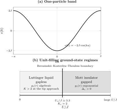
Left: exact one-particle dispersion with bandwidth $4J$. Right: the repulsive, homogeneous, unit-filled chain changes from a gapless Luttinger liquid to a Mott insulator near $U_c/J\simeq3.3$; the numerical value is convention-specific and the transition is BKT, not a simple power-law critical point.

Zero-Temperature Regimes

Incommensurate filling

For repulsive finite $U/J$ away from integer filling, the clean chain is generically compressible and gapless. Its long-distance sector is a one-component Luttinger liquid. There is no ordinary quasiparticle pole and no true interacting Bose condensate in the infinite one-dimensional ground state, but phase correlations remain algebraic.

Integer filling

At $\nu=n_0\in\mathbb Z_{>0}$, lattice Umklapp can pin the density field. Weak interaction leaves a gapless Luttinger liquid; sufficiently strong interaction produces an incompressible Mott insulator with a finite charge gap and exponentially decaying one-body correlations.

At unit filling for the standard nearest-neighbor Hamiltonian used here, high-accuracy numerical studies place the tip near

$$\frac{U_c}{J} \simeq 3.3.$$

This is a numerical estimate, not an exact constant. BKT logarithms, boundary conditions, truncation, and the chosen estimator explain why finite-size studies can produce visibly different apparent values.

Tip versus lobe side

At fixed integer density, crossing the lobe tip by changing $U/J$ gives the commensurate BKT transition with dynamical exponent $z=1$. Crossing a side by changing $\mu$ creates dilute particles or holes and has the generic density-driven structure with $z=2$. Quoting one “Bose–Hubbard critical exponent” without the trajectory is therefore incomplete.

Finite temperature

At any nonzero temperature, an infinite one-dimensional short-range chain has a finite thermal correlation length. The zero-temperature Luttinger liquid and Mott insulator still organize crossovers, response, and finite-system behavior, but their ground-state correlation laws should not be applied unchanged at arbitrarily long thermal distances.

Luttinger-Liquid Diagnostics

Use the convention

$$H_{\mathrm{LL}} = \frac{\hbar v}{2\pi} \int dx\, \left[ K(\partial_x\theta)^2 + \frac1K(\partial_x\phi)^2 \right].$$

In this normalization, the one-body correlation has leading behavior

$$g_1(r) = \langle b_{j+r}^\dagger b_j\rangle \sim A_0 r^{-1/(2K)},$$

while the connected density correlation is

$$\begin{aligned} \langle\delta n_{j+r}\delta n_j\rangle \sim{}& -\frac{K}{2\pi^2r^2} \\ &+ A_1 \frac{\cos(2\pi\nu r)}{r^{2K}} +\cdots. \end{aligned}$$

Consequently, for small dimensionless lattice momentum $q$,

$$S(q) \sim \frac{K\lvert q\rvert}{2\pi}.$$

Several observables should yield the same $K$ and sound velocity $v$ over one infrared window. Agreement from only one fit can hide boundary, cutoff, or subleading-correction bias.

Universal commensurate criterion

At simplest integer commensurability, the leading lattice perturbation is proportional to $\cos(2\phi)$. In the convention above it becomes marginal at

$$K_c=2.$$

The one-body exponent is therefore $1/4$ at the transition, up to logarithmic corrections. Deeper in the hard-core incommensurate liquid, $K=1$; no contradiction occurs because the unit-filled hard-core endpoint is already the filled, gapped state.

BKT gap opening

On the insulating side near the tip, the charge gap has the essential-singularity form

$$\Delta_c \sim A \exp\left[ -\frac{B}{\sqrt{U/U_c-1}} \right],$$

where $A$ and $B$ are nonuniversal. There is no finite ordinary exponent $\nu$ describing this divergence. Polynomial extrapolation of a few finite gaps is therefore unreliable near the tip.

Finite-Size Energy Diagnostics

Let $E_0(L,N)$ be the canonical ground-state energy. Define

$$\begin{aligned} \mu_+(L,N) &= E_0(L,N+1)-E_0(L,N), \\ \mu_-(L,N) &= E_0(L,N)-E_0(L,N-1), \\ \Delta_c(L,N) &= \mu_+-\mu_-. \end{aligned}$$

Equivalently,

$$\Delta_c(L,N) = E_0(L,N+1) +E_0(L,N-1) -2E_0(L,N).$$

In a Mott phase, $\Delta_c(L)$ approaches a nonzero limit. In a Luttinger liquid with periodic boundaries,

$$\Delta_c(L) = \frac{\pi\hbar v}{KL} + o(L^{-1})$$

under the stated field normalization. Boundary and logarithmic corrections can be substantial.

The gap should be analyzed together with compressibility, correlation exponents, stiffness or twist curvature, and entanglement scaling. A single positive finite-size gap does not establish an insulator.

Observables

One-body density matrix and momentum distribution

Define

$$G_{j\ell} = \langle b_j^\dagger b_\ell\rangle.$$

For a translation-invariant ring,

$$n(k) = \sum_r e^{-ikr a}g_1(r).$$

In the interacting Luttinger liquid, the $k=0$ peak grows subextensively with $L$. In the Mott phase it saturates on the scale set by the finite correlation length.

Density structure factor

With $\delta n_j=n_j-\nu$,

$$S(q) = \frac1L \sum_{j,\ell} e^{-iq a(j-\ell)} \langle\delta n_j\delta n_\ell\rangle.$$

Its small-$q$ slope gives $K$ in the gapless phase. In a gapped Mott state, $S(q)$ is analytic and begins quadratically under standard short-range conditions.

Onsite pair density

$$d = \frac1{2L} \sum_j \langle n_j(n_j-1)\rangle = \frac1L \frac{\partial E_0}{\partial U}.$$

This local observable tracks multiple occupancy but is not by itself an order parameter for the Mott transition.

Compressibility and twist response

The zero-temperature compressibility is obtained from the curvature of $E_0(N)$ or from $\partial\nu/\partial\mu$. A Mott phase has zero bulk compressibility. On a ring, the curvature of $E_0(\Phi)$ probes coherent transport. Its prefactor depends on whether one reports helicity modulus, Drude weight, or superfluid fraction, so the definition must accompany the number.

Entanglement

The gapless chain has central charge $c=1$. For a periodic ring, the leading interval entropy is

$$S(\ell) = \frac c3 \ln\left[ \frac{L}{\pi a_0} \sin\left(\frac{\pi\ell}{L}\right) \right] +s_1+\cdots,$$

where $a_0$ is a short-distance cutoff. Open boundaries halve the logarithmic coefficient and introduce stronger boundary oscillations. The canonical derivation and fitting cautions live in Entanglement Entropy in Many-Body Systems.

Physical Phenomena

• Interaction-driven localization: onsite repulsion can create a Mott gap without disorder.
• Quasi-long-range phase coherence: the gapless interacting chain has algebraic, not constant, one-body correlations.
• Bosonic enhancement: particles and holes propagate with occupation-dependent amplitudes.
• BKT criticality: the commensurate tip has an essential correlation-length singularity and logarithmic drift.
• Fermionization: hard-core energies and density observables map to free fermions, while bosonic coherence retains a nonlocal string.
• Quantum-number fractionalization in the infrared: low-energy density waves replace a simple particle quasiparticle description.
• Collapse for attraction: the unconstrained attractive chain lacks a stable extensive thermodynamic limit.

Minimal Worked Example: One Boson on a Ring

For $N=1$, the interaction vanishes. On an untwisted $L$-site ring,

$$\lvert k_m\rangle = \frac1{\sqrt L} \sum_{j=1}^{L} e^{ik_m aj} \lvert j\rangle,$$

with

$$k_m = \frac{2\pi m}{La}, \qquad E_m = -2J\cos(k_m a).$$

The ground state at $\Phi=0$ is uniform and has $E_0=-2J$. With a twist, replace $2\pi m$ by $2\pi m+\Phi$. Level crossings as $\Phi$ varies are finite-ring momentum-sector crossings, not interaction-driven phase transitions.

Finite-Cluster Benchmark: Open L = 3, N = 2

This dossier uses a six-state check that is independent of the dimer contract. Take open bonds $(1,2)$ and $(2,3)$, set $J=1$, $U=2$, and order the basis as

$$\bigl\{ \lvert2,0,0\rangle, \lvert1,1,0\rangle, \lvert1,0,1\rangle, \lvert0,2,0\rangle, \lvert0,1,1\rangle, \lvert0,0,2\rangle \bigr\}.$$

For symbolic $J,U$, the matrix is

$$H = \begin{pmatrix} U&-\sqrt2J&0&0&0&0\\ -\sqrt2J&0&-J&-\sqrt2J&0&0\\ 0&-J&0&0&-J&0\\ 0&-\sqrt2J&0&U&-\sqrt2J&0\\ 0&0&-J&-\sqrt2J&0&-\sqrt2J\\ 0&0&0&0&-\sqrt2J&U \end{pmatrix}.$$

Reflection blocks

Reflection exchanges sites $1$ and $3$. The odd block is

$$H_- = \begin{pmatrix} U&-\sqrt2J\\ -\sqrt2J&0 \end{pmatrix},$$

with energies

$$E_{-,\pm} = \frac{U\pm\sqrt{U^2+8J^2}}{2}.$$

The even sector contains one dark eigenvalue $E=U$. Its other three energies are the roots of

$$p(E) = E^3-UE^2-8J^2E+2UJ^2.$$

At $J=1$, $U=2$, the sorted spectrum is

$$\begin{array}{c|c} E & \text{reflection parity}\\ \hline -2.279452315768606 & +\\ -0.732050807568877 & -\\ 0.459362941393819 & +\\ 2.000000000000000 & +\\ 2.732050807568877 & -\\ 3.820089374374788 & + \end{array}$$

For the ground state,

$$\left\langle \frac12\sum_{j=1}^{3}n_j(n_j-1) \right\rangle_0 = 0.191308218635467\ldots.$$

This equals $\partial E_0/\partial U$. For a root of $p(E)=0$,

$$\frac{\partial E}{\partial U} = \frac{E^2-2J^2} {3E^2-2UE-8J^2}.$$

Matrix invariants

Before diagonalization, verify

$$\begin{aligned} \operatorname{Tr}H &=3U, \\ \operatorname{Tr}H^2 &=3U^2+20J^2, \\ \det H &=4U^2J^4. \end{aligned}$$

At the benchmark point these are $6$, $32$, and $16$. This cluster checks basis enumeration, two distinct open bonds, unit and $\sqrt2$ hopping factors, reflection symmetry, eigenvectors, and a Feynman–Hellmann observable. It is intentionally not labeled MB-B005, which belongs to the physical two-site dimer.

Numerical Methods and Error Controls

Exact diagonalization

Use fixed-$N$ sectors and, for periodic rings, translation and inversion blocks. Report the basis order, bond list, boundary twist, local cutoff if any, and residual norms. Small clusters cannot resolve BKT scaling by themselves.

Matrix-product states and DMRG

Open-boundary DMRG is a standard high-accuracy method for this chain. Converge both bond dimension and $n_{\max}$. In the Luttinger liquid, finite entanglement creates an effective correlation length; near the BKT point, logarithmic corrections make naive power-law fits drift.

Quantum Monte Carlo

The repulsive, unfrustrated model with real hopping admits efficient worldline methods. Winding-number estimators access stiffness on periodic space-time geometries. Autocorrelation, temporal discretization if present, and finite-size scaling remain part of the error budget.

Cross-method checks

A robust calculation should reproduce:

• the $U=0$ cosine band and many-boson ground energy;
• atomic-limit occupations and gaps;
• the hard-core free-fermion energy density;
• Feynman–Hellmann pair density;
• consistent $K$ from structure factor, compressibility/stiffness, and correlations;
• the six-state open-chain benchmark above.

Variants and Handoffs

Traps and inhomogeneity

A term $\sum_jV_jn_j$ breaks translation symmetry and can create coexisting density regions. Local-density reasoning is approximate near boundaries and over short traps. The general trapped-lattice interpretation belongs in the Bose–Hubbard Model article.

Nearest-neighbor interaction

Adding $V\sum_jn_jn_{j+1}$ produces the extended Bose–Hubbard chain, with charge-density-wave, Haldane-insulator, and other regimes depending on filling and parameters. Those are not phases of the minimal onsite-only Hamiltonian.

Disorder

Random onsite energies can create a compressible Bose glass and change the transition structure. A clean Mott-to-Luttinger-liquid statement should not be transferred to the disordered chain.

Flux, driving, and dissipation

Complex hopping, periodic drive, loss, or dephasing modifies symmetry and transport. The closed, static, real-hopping chain remains the reference model.

Two modes

The Bose–Hubbard Dimer owns finite two-mode Josephson physics, exact $N=2$ formulas, and the MB-B005 contract. It should not be inferred by setting $L=2$ in a periodic chain sum without checking bond multiplicity.

Common Mistakes

Calling the generic soft-core chain integrable

$U=0$ and the hard-core projection are exactly solvable. Generic finite $U/J$ is not the Lieb–Liniger model and has no standard Bethe-ansatz solution.

Double-counting the L = 2 bond

Modulo indexing can turn one physical link into two parallel contributions. Use an explicit graph for short systems.

Omitting bosonic square roots

Hopping amplitudes depend on both departure and arrival occupations. Constant amplitudes fail as soon as multiple occupancy appears.

Equating one-dimensional superfluidity with true condensation

At interacting zero-temperature gapless points, $g_1(r)$ decays algebraically and the largest natural occupation is subextensive. Finite systems can still display a sharp momentum peak and nonzero stiffness.

Inferring a Mott phase from integer density alone

Integer filling is necessary for the clean onsite model’s Mott state but not sufficient. The charge gap and compressibility distinguish the weak-coupling Luttinger liquid from the Mott insulator.

Fitting the BKT point with an ordinary power law

The correlation length has an essential singularity and finite-size corrections are logarithmic. Apparent crossings drift slowly.

Treating hard-core boson coherence as free-fermion coherence

The spectra and density observables map simply. Bosonic creation operators carry Jordan–Wigner strings, so their off-diagonal correlations do not equal fermionic Green functions.

Ignoring local-cutoff convergence

An energy can appear converged while pair density, tails of $P(n_j)$, or spectral weights remain cutoff-sensitive.

Exercises

1. Count the fixed-number basis

Derive $\dim\mathcal H_{N,L}=\binom{N+L-1}{N}$ and evaluate it for $L=6$, $N=6$.

Solution

A basis state is a weak composition of $N$ into $L$ nonnegative integers. Place $L-1$ separators among $N+L-1$ positions, giving

$$\dim\mathcal H_{N,L} = \binom{N+L-1}{L-1} = \binom{N+L-1}{N}.$$

For $L=N=6$,

$$\dim\mathcal H_{6,6} = \binom{11}{6} =462.$$

2. Derive the twisted one-particle spectrum

For a ring with $b_{L+1}=e^{i\Phi}b_1$, derive the allowed momenta and energies.

Solution

A plane wave has amplitude $e^{ikaj}$. The boundary condition requires

$$e^{ikLa}=e^{i\Phi},$$

so

$$k_m = \frac{2\pi m+\Phi}{La}.$$

Acting with nearest-neighbor hopping gives

$$E_m = -J \left( e^{ik_ma}+e^{-ik_ma} \right) = -2J\cos(k_ma).$$

3. Obtain the strong-coupling particle and hole bands

Start from the integer product state with $n_0$ bosons per site. Show why an added particle hops with amplitude $-J(n_0+1)$ while a hole hops with amplitude $-Jn_0$.

Solution

Let the extra particle occupy site $j$, whose occupation is $n_0+1$. Moving it to a neighboring site applies $b_{j+1}^\dagger b_j$ and gives

$$\sqrt{n_0+1}\sqrt{n_0+1} =n_0+1.$$

The effective nearest-neighbor matrix element is therefore $-J(n_0+1)$. A hole state has occupation $n_0-1$ at one site. Moving the hole is equivalent to moving one background boson into it, with factor

$$\sqrt{n_0}\sqrt{n_0} =n_0.$$

Fourier transformation of these effective tight-binding problems gives the two dispersions stated in the text.

4. Recover the hard-core energy density

Map the hard-core chain at filling $0\le\nu\le1$ to free fermions and derive $E_0/L$ in the thermodynamic limit.

Solution

The mapped fermions fill momenta from $-k_F$ to $k_F$, with

$$k_Fa=\pi\nu.$$

Using $\epsilon(k)=-2J\cos(ka)$,

$$\begin{aligned} \frac{E_0}{L} &= \frac{a}{2\pi} \int_{-k_F}^{k_F} dk\, [-2J\cos(ka)] \\ &= -\frac{2J}{\pi} \sin(\pi\nu). \end{aligned}$$

Differentiating the dispersion at $k_F$ gives $v=2Ja\sin(\pi\nu)/\hbar$.

5. Interpret a finite charge gap

A periodic finite-size calculation in a gapless regime gives $\Delta_c(L)=0.18J$ at $L=32$ and $0.091J$ at $L=64$. Does either positive number demonstrate a Mott gap?

Solution

No. The values approximately halve when $L$ doubles, which is consistent with the Luttinger-liquid scaling

$$\Delta_c(L) \propto \frac1L.$$

A Mott claim requires an extrapolation to a positive limit and consistency with incompressibility and exponential correlations. Near a BKT point, logarithmic corrections require more than a two-size fit.

6. Reconstruct the three-site parity blocks

Using the six-state benchmark basis, construct reflection-even and reflection-odd combinations. Show that the odd eigenvalues are $(U\pm\sqrt{U^2+8J^2})/2$ and identify the even dark state at energy $U$.

Solution

Define

$$\begin{aligned} \lvert D_\pm\rangle &= \frac{ \lvert2,0,0\rangle \pm \lvert0,0,2\rangle }{\sqrt2}, \\ \lvert B_\pm\rangle &= \frac{ \lvert1,1,0\rangle \pm \lvert0,1,1\rangle }{\sqrt2}. \end{aligned}$$

The odd basis $\{\lvert D_-\rangle,\lvert B_-\rangle\}$ gives

$$H_- = \begin{pmatrix} U&-\sqrt2J\\ -\sqrt2J&0 \end{pmatrix},$$

whose quadratic characteristic equation yields the stated roots.

In the even doublon subspace, the combination

$$\lvert D_{\mathrm{dark}}\rangle = \frac{ \sqrt2\lvert D_+\rangle - \lvert0,2,0\rangle }{\sqrt3}$$

has zero hopping matrix element into $\lvert B_+\rangle$. Because every component has one onsite pair, it is an eigenstate with $E=U$.

Cross-Links

• Model Encyclopedia Overview – dossier contract and exactness labels.
• Bose–Hubbard Model – canonical general-lattice treatment and optical-lattice reduction.
• Bose–Hubbard Dimer – exact two-mode finite system.
• Boundary Conditions on Lattices – twists, graph closure, and finite-size conventions.
• Jordan–Wigner Transformation – parity-sensitive hard-core mapping.
• Luttinger Liquid Preview – field normalization, operators, and commensurate perturbations.
• Quantum Phase Transitions – lobe sides, tips, and BKT interpretation.
• Exact Diagonalization Preview – sparse finite-sector construction.
• DMRG Preview – matrix-product-state convergence in one dimension.
• Finite-Size Scaling in Numerics – extrapolation and correction terms.
• Bose–Hubbard Model Card – compact reference entry.

References

• H. A. Gersch and G. C. Knollman, “Quantum Cell Model for Bosons,” Physical Review 129, 959–967 (1963), doi:10.1103/PhysRev.129.959.
• M. P. A. Fisher, P. B. Weichman, G. Grinstein, and D. S. Fisher, “Boson Localization and the Superfluid-Insulator Transition,” Physical Review B 40, 546–570 (1989), doi:10.1103/PhysRevB.40.546.
• T. D. Kühner and H. Monien, “Phases of the One-Dimensional Bose–Hubbard Model,” Physical Review B 58, R14741–R14744 (1998), doi:10.1103/PhysRevB.58.R14741.
• D. Jaksch, C. Bruder, J. I. Cirac, C. W. Gardiner, and P. Zoller, “Cold Bosonic Atoms in Optical Lattices,” Physical Review Letters 81, 3108–3111 (1998), doi:10.1103/PhysRevLett.81.3108.
• T. D. Kühner, S. R. White, and H. Monien, “One-Dimensional Bose–Hubbard Model with Nearest-Neighbor Interaction,” Physical Review B 61, 12474–12489 (2000), doi:10.1103/PhysRevB.61.12474.
• M. A. Cazalilla, “Bosonizing One-Dimensional Cold Atomic Gases,” Journal of Physics B: Atomic, Molecular and Optical Physics 37, S1–S47 (2004), doi:10.1088/0953-4075/37/7/051.
• M. A. Cazalilla, R. Citro, T. Giamarchi, E. Orignac, and M. Rigol, “One Dimensional Bosons: From Condensed Matter Systems to Ultracold Gases,” Reviews of Modern Physics 83, 1405–1466 (2011), doi:10.1103/RevModPhys.83.1405.
• S. Ejima, H. Fehske, F. Gebhard, K. zu Münster, M. Knap, E. Arrigoni, and W. von der Linden, “Characterization of Mott-Insulating and Superfluid Phases in the One-Dimensional Bose–Hubbard Model,” Physical Review A 85, 053644 (2012), doi:10.1103/PhysRevA.85.053644.
• T. G. Kiely and E. J. Mueller, “Superfluidity in the One-Dimensional Bose–Hubbard Model,” Physical Review B 105, 134502 (2022), doi:10.1103/PhysRevB.105.134502.