Finite-Size Scaling in Numerics

Finite-size scaling is the controlled inference of thermodynamic behavior from a declared sequence of finite systems. It is not the act of drawing a smooth curve through a few values of the site count. A defensible calculation specifies which geometries, boundary conditions, symmetry sectors, aspect ratios, observables, and numerical tolerances define the sequence; separates numerical error from physical finite-size effects; and tests whether more than one asymptotic explanation is compatible with the accessible sizes.

Use Finite-Size Effects first to identify the physical mechanism—quantization, boundaries, shells, commensurability, correlation cutoffs, traps, or finite-time resolution. This page begins when that diagnosis must be turned into a numerical extrapolation with an explicit error model.

For a finite-system datum $\widehat O_L$, the logical structure is

$$\widehat O_L = O_L +\delta O_L^{\mathrm{num}}, \qquad O_L = O_\infty +\delta O_L^{\mathrm{fs}}.$$

The first correction belongs to the solver. The second belongs to the finite physical system. Reducing one does not automatically control the other.

Purpose and canonical scope

This page owns the practical numerical protocol for connecting data at finite $L$ to claims about gaps, order, correlation lengths, critical points, and exponents. It emphasizes what must be recorded, which quantities should be compared, how competing scaling regimes can be distinguished, and what robustness checks support an extrapolation.

The mathematical theory of scaling fields, exponent identities, universality, data collapse, and corrections to scaling has its canonical treatment in Critical Exponents and Scaling. The Critical Exponent Glossary is the quick reference for fitting powers, scaling dimensions, and assumption checks. The definition of a limiting sequence belongs to The Thermodynamic Limit. Definitions of order parameters, connected correlations, and structure factors are also developed at their canonical homes.

The numerical question here is narrower and more operational:

Given controlled data on a finite family, which thermodynamic statements are supported, which remain hypotheses, and what additional sizes or observables would discriminate between them?

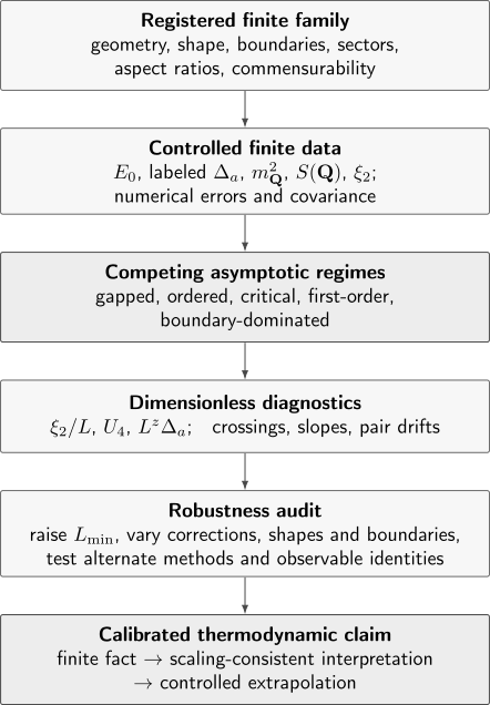
A finite-size conclusion is an evidence chain. Geometry, boundaries, sectors, and numerical tolerances determine the family; raw observables constrain candidate regimes; dimensionless ratios and robustness tests determine how strong the final claim may be.

The finite-system claim ladder

It helps to separate statements that are often compressed into the phrase “the numerics show.”

1. Exact finite-system fact. For a specified Hamiltonian matrix and sector, a theorem or exact diagonalization gives a value without extrapolation.
2. Numerically controlled finite-system estimate. A solver returns a value with convergence evidence, such as a residual, variance, truncation extrapolation, or Monte Carlo uncertainty.
3. Observed finite-size trend. A registered sequence displays monotonicity, a crossing, a power-like window, or convergence toward an apparent limit.
4. Scaling-consistent interpretation. Several observables agree with a gapped, ordered, critical, or first-order hypothesis over stable fit windows.
5. Thermodynamic conclusion. Extrapolation remains stable under corrections, omitted sizes, geometry changes, and plausible competing models.
6. Universality claim. Critical exponents, amplitude combinations, or scaling functions agree across microscopic realizations after the required metric factors and corrections are handled.

Each rung requires more evidence than the preceding one. A clean crossing is a useful estimator, but by itself it is not a universality result.

Register the finite family

Before fitting anything, define the family of finite problems. A useful record is

$$\mathcal F_L = \bigl( \Lambda_L,\, \mathcal B_L,\, \mathcal S_L,\, \boldsymbol\alpha_L,\, H_L,\, \mathcal O_L \bigr),$$

where $\Lambda_L$ is the geometry, $\mathcal B_L$ the boundary condition, $\mathcal S_L$ the symmetry sector or ensemble, $\boldsymbol\alpha_L$ the aspect-ratio data, $H_L$ the finite Hamiltonian, and $\mathcal O_L$ the observable definition and normalization.

What does the size mean?

For an isotropic $d$-dimensional lattice with $n_{\mathrm u}$ sites per unit cell,

$$N(L) = n_{\mathrm u}L^d$$

is often adequate. But $L=N^{1/d}$ is not a universal definition. On cylinders, ladders, anisotropic clusters, irregular graphs, momentum grids, and tensor-network geometries, several lengths may matter:

$$L_x,\quad L_y,\quad \ldots,\quad r_{xy}=\frac{L_x}{L_y}.$$

Scaling comparisons should hold the relevant shape ratios fixed. A sequence of $4\times L$, $6\times L$, and $8\times L$ cylinders is not a single isotropic sequence merely because each member has a site count.

When clusters have different shapes, report both $N$ and the linear dimensions. If an effective length is used, define it. For example,

$$L_{\mathrm{vol}} = \left( \frac{N}{n_{\mathrm u}} \right)^{1/d}$$

captures volume but not anisotropy.

Geometry and commensurability

A cluster must be able to represent the candidate ordering wavevector and unit cell. If a phase is expected at wavevector $\mathbf Q$, then a periodic cluster should satisfy

$$e^{i\mathbf Q\cdot\mathbf L_\mu}=1$$

along every periodic primitive direction $\mathbf L_\mu$. Incommensurate clusters can frustrate the order, shift low-energy momenta, or create a false drift. Excluding such clusters after seeing the answer invites selection bias; classify the compatible families in advance.

Cluster shape also changes the spectrum of the smallest nonzero momentum. For a rectangular periodic lattice,

$$\begin{aligned} \mathbf q_{\min}^{(x)} &= \left(\frac{2\pi}{L_x},0,\ldots\right), \\ \mathbf q_{\min}^{(y)} &= \left(0,\frac{2\pi}{L_y},\ldots\right). \end{aligned}$$

If correlations are anisotropic, the corresponding correlation-length estimators need not agree.

Boundary conditions are part of the model sequence

Open, periodic, antiperiodic, twisted, cylindrical, and symmetry-breaking boundaries produce different leading corrections. A boundary choice may also introduce edge states or remove momenta needed to label excitations. Therefore one should not merge them into a single fit by replacing each cluster with an effective $L$.

For open boundaries, a local bulk observable and a whole-system average can converge at different rates. The boundary fraction scales as

$$\frac{N_{\partial}}{N} \sim \frac{L^{d-1}}{L^d} = \frac{1}{L},$$

so a surface contribution can dominate the leading correction even when bulk correlations are short-ranged.

Symmetry sectors define spectral identities

A finite-size gap must be labeled by the quantum numbers of both levels:

$$\Delta_{\lambda\leftarrow 0}(L) = E_{0,\lambda}(L) -E_{0,\lambda_0}(L),$$

or, within the ground-state sector,

$$\Delta_{n,\lambda_0}(L) = E_{n,\lambda_0}(L) -E_{0,\lambda_0}(L).$$

These are different observables. The lowest state in another parity sector may be a tunneling partner, while the first state at nonzero momentum may be a propagating mode. See Symmetry Sectors in Many-Body Numerics for sector construction and state tracking.

Quantum aspect ratios

Ground-state algorithms introduce additional scales. A finite-temperature or projector calculation has an imaginary-time extent $\beta$, and a critical system with dynamic exponent $z$ requires a controlled spacetime aspect ratio,

$$\frac{\beta}{L^z} = \text{constant},$$

or a demonstrated $\beta\to\infty$ limit at each $L$. Holding $\beta/L$ fixed silently assumes $z=1$. If $z$ is under investigation, repeat the analysis over plausible choices or establish ground-state convergence independently.

Finite-entanglement, bond-dimension, basis-cutoff, walker-population, and sampling scales play analogous roles. They belong in the registered family whenever they remain physically active.

Separate numerical error from finite-size drift

Suppose the solver returns $\widehat O_L$ with estimated numerical uncertainty $\sigma_L$. An asymptotic model $f(L;\boldsymbol\theta)$ should be tested against

$$\widehat O_L = f(L;\boldsymbol\theta) +\varepsilon_L^{\mathrm{num}} +\varepsilon_L^{\mathrm{model}}.$$

The first residual is controlled by solver diagnostics. The second represents neglected finite-size terms and possible model misspecification. A tiny $\sigma_L$ can make an inadequate scaling ansatz fail more visibly; it does not make that ansatz correct.

Useful numerical controls include:

• eigenpair residuals and energy variances for exact diagonalization or Lanczos;
• discarded weight, variance, and bond-dimension extrapolation for matrix-product states;
• autocorrelation-aware standard errors and equilibration tests for Monte Carlo;
• Trotter-step, projection-time, and population extrapolations where applicable;
• agreement between independent implementations or methods on overlapping sizes.

The Computational Many-Body Overview develops the full error ledger. A fit should not use a point whose numerical bias is comparable to the finite-size trend being interpreted.

Correlated data

Finite-size data may share random numbers, reweighting samples, fitted ground states, normalization estimates, or common calibration parameters. Then the covariance matrix

$$C_{ij} = \operatorname{Cov} \left( \widehat O_{L_i}, \widehat O_{L_j} \right)$$

matters. For residual vector $\mathbf r$, the appropriate quadratic form is

$$\chi^2 = \mathbf r^{\mathsf T} C^{-1} \mathbf r,$$

provided $C$ is itself estimated reliably. A nearly singular empirical covariance matrix may require blocked resampling, a carefully documented regularization, or a reduced set of independent summaries. Treating strongly correlated points as independent generally overstates precision.

Ground-state energy scaling

The total ground-state energy is extensive, so the intensive quantity

$$e_0(L) = \frac{E_0(L)}{N(L)}$$

is usually the object extrapolated to the thermodynamic energy density $e_\infty$.

For an open, regular $d$-dimensional region, a generic decomposition is

$$E_0(L) = e_\infty L^d +e_{\mathrm s}L^{d-1} +e_{\mathrm e}L^{d-2} +\cdots,$$

where surface, edge, and corner terms depend on geometry and conventions. Dividing by $L^d$ gives

$$e_0(L) = e_\infty +\frac{e_{\mathrm s}}{L} +\frac{e_{\mathrm e}}{L^2} +\cdots.$$

Periodic boundaries remove a physical surface, but they do not guarantee a pure polynomial in $1/L$. In a short-range gapped phase, wrapping corrections can be exponentially small,

$$e_0(L)-e_\infty \sim L^p e^{-L/\xi},$$

possibly together with analytic corrections. At a quantum critical point, universal and nonuniversal power-law terms may coexist. Their exponents depend on dimension, dynamic scaling, shape, and boundary condition.

Two cautions are essential:

1. A straight line in $1/L$ is physically motivated for many open-boundary energy densities, but not for every geometry.
2. A highly accurate estimate of $e_\infty$ does not by itself identify a phase. Energies are often less discriminating than gaps, correlations, or symmetry-resolved observables.

Increment estimators

If a sequence grows by a fixed unit, an energy increment can reduce the leading extensive contribution:

$$\mu_L = \frac{ E_0(L+\delta L)-E_0(L) }{ N(L+\delta L)-N(L) }.$$

Under suitable regularity, $\mu_L\to e_\infty$. But adjacent increments share energy estimates and are statistically correlated. They can also amplify oscillatory shell or parity effects. The estimator must be analyzed as a new observable, not assumed to be superior.

Gap scaling

Gap scaling is powerful only after the excitation has a stable physical identity. Record momentum, internal quantum numbers, boundary localization, and state-tracking diagnostics alongside every energy difference.

Common asymptotic regimes

Several physically distinct scales can appear in one spectrum.

Bulk gapped phase. A stable bulk excitation approaches

$$\begin{gathered} \Delta_{\mathrm{bulk}}(L) = \Delta_\infty +aL^p e^{-L/\xi_\Delta} +\cdots, \\ \Delta_\infty>0. \end{gathered}$$

A power correction can replace or accompany the exponential term, depending on boundaries and the observable.

Continuous quantum critical point. For a critical excitation whose energy is controlled by the longest wavelength,

$$\Delta_a(L,g_c) = L^{-z} \left[ c_a +b_aL^{-\omega} +\cdots \right].$$

The coefficient $c_a$ depends on the excitation, geometry, velocity conventions, and boundaries. The exponent $z$ belongs to the critical theory.

Discrete symmetry breaking. A finite symmetry eigenstate can have an exponentially small splitting to its symmetry partner,

$$\Delta_{\mathrm{cat}}(L) \sim L^p e^{-\sigma L^d},$$

as a representative short-range form, while the local bulk excitation gap remains nonzero. The tunneling action and prefactor depend on dynamics, geometry, and boundaries, so the displayed volume exponent is not a universal fitting law. Calling the cat-state splitting “the gap” would incorrectly classify the ordered phase as gapless.

Continuous symmetry breaking. A finite system can exhibit an Anderson tower of global rotations,

$$\Delta_{\mathrm{tower}}(L) \sim \frac{1}{L^d},$$

and Goldstone excitations at the smallest nonzero momentum,

$$\Delta_{\mathrm G}(L) \sim \frac{v}{L}$$

for a linearly dispersing mode. These are different level families. Their symmetry and momentum labels are the diagnostic. The canonical physical interpretation belongs to Spontaneous Symmetry Breaking.

First-order transition. Near phase coexistence, avoided crossings and tunneling can generate exponentially small gaps whose scale is strongly boundary- and geometry-dependent. Such a gap does not imply a continuous critical point with very large $z$.

Boundary mode. Open systems may have edge or end-state splittings that vanish exponentially with system length even though the bulk remains gapped. Spatial profiles and boundary-condition comparisons are necessary.

Scaled gaps

Given a candidate $z$, define

$$R_{\Delta,a}(L,g) = L^z\Delta_a(L,g).$$

At a continuous critical point, $R_{\Delta,a}$ may approach a size-independent function at fixed shape and boundary condition. Crossings between $L$ and $sL$ can estimate $g_c$, but corrections shift the crossings.

An effective exponent from adjacent sizes is

$$z_{\mathrm{eff}}(L;s) = - \frac{ \ln\!\left[ \Delta(sL)/\Delta(L) \right] }{ \ln s }.$$

If

$$\Delta(L) = cL^{-z} \left( 1+bL^{-\omega} +\cdots \right),$$

then $z_{\mathrm{eff}}$ approaches $z$ only after the correction becomes small. A plateau over two size pairs is evidence worth reporting, not proof of asymptotia.

State tracking

Ordering energies by index can misidentify a gap when levels cross. Track states using all available information:

• exact symmetry labels;
• momentum and point-group quantum numbers;
• overlap with the state at a nearby coupling;
• matrix elements of diagnostic operators;
• spatial localization and entanglement structure;
• continuity under boundary twists.

In a Lanczos calculation, residual convergence of both energies is necessary but does not establish that the two Ritz vectors represent the same excitation branch across sizes. The numerical method is developed in Lanczos Method Preview.

Order-parameter scaling

Let a local operator $O_j$ diagnose order at wavevector $\mathbf Q$. Define the extensive Fourier component

$$M_{\mathbf Q} = \sum_{j=1}^{N} e^{i\mathbf Q\cdot\mathbf r_j} O_j.$$

With the normalization

$$m_{\mathbf Q}^2(L) = \frac{ \left\langle M_{\mathbf Q}^{\dagger}M_{\mathbf Q} \right\rangle }{ N^2 },$$

and

$$S(\mathbf Q) = \frac{ \left\langle M_{\mathbf Q}^{\dagger}M_{\mathbf Q} \right\rangle }{ N },$$

the two quantities obey

$$m_{\mathbf Q}^2(L) = \frac{S(\mathbf Q)}{N}.$$

This identity is normalization-dependent, so every numerical paper or notebook should state its Fourier convention.

Why the squared order parameter is needed

In a finite system that preserves the symmetry,

$$\langle M_{\mathbf Q}\rangle = 0$$

can hold throughout an ordered phase. The vanishing one-point function reflects the finite symmetry eigenstate, not the absence of thermodynamic order. The squared moment, long-distance correlator, structure factor, or full order-parameter distribution remains informative.

Under the normalization above:

Ordered phase

$$m_{\mathbf Q}^2(L) \longrightarrow m_\infty^2>0.$$

Short-range disordered phase

$$S(\mathbf Q) \longrightarrow \text{constant}, \qquad m_{\mathbf Q}^2(L) \sim \frac{1}{N}.$$

Continuous critical point

$$m_{\mathbf Q}^2(L,g_c) \sim L^{-2\beta/\nu} \left( a_0+a_1L^{-\omega}+\cdots \right),$$

for the conventional order-parameter exponents and a compatible spacetime aspect ratio.

These leading forms are candidates, not automatic fit functions. Goldstone fluctuations, dangerously irrelevant variables, anisotropy, long-range interactions, and boundaries can alter the useful correction structure.

Binder ratios

For a scalar order parameter with an Ising-like convention, one common dimensionless cumulant is

$$U_4 = 1- \frac{ \langle M^4\rangle }{ 3\langle M^2\rangle^2 }.$$

Different symmetry groups and normalizations use different constants or moment ratios. Quote the definition, not only the symbol. At a continuous transition, $U_4$ can have size crossings; near a first-order transition, its distribution-sensitive behavior can be more complicated and may include pronounced nonmonotonicity.

Because fourth moments are noise-sensitive, a Binder crossing should be accompanied by autocorrelation analysis, resampling, and the underlying order-parameter distribution when feasible.

Correlation-length diagnostics

The exponential correlation length and the second-moment estimator are related but not identical finite-size observables. Begin with the connected structure factor around the ordering wavevector $\mathbf Q$. On a periodic lattice with lattice spacing set to one, a common estimator is

$$\begin{aligned} \xi_2 &= \frac{1}{ 2\sin\!\left( \lvert\mathbf q_{\min}\rvert/2 \right) } \\ &\quad\times \sqrt{ \frac{ S_c(\mathbf Q) }{ S_c(\mathbf Q+\mathbf q_{\min}) } -1 }. \end{aligned}$$

This follows from matching the smallest available momenta to the leading lattice form of a smooth, isotropic peak along the chosen direction. The dimensionless ratio

$$R_\xi = \frac{\xi_2}{L}$$

is often used as a crossing observable.

The formula requires care:

• $S_c$ must use the connected correlator if the one-point function is nonzero;
• $\mathbf q_{\min}$ and $L$ must refer to the same direction;
• an anisotropic system can require separate $\xi_x/L_x$ and $\xi_y/L_y$;
• an incommensurate or multi-peaked structure factor may invalidate the one-peak estimate;
• finite periodic data can make the expression noisy or negative within uncertainty;
• open boundaries break the direct momentum-space derivation.

For open systems, alternatives include fits to bulk-window correlations, real-space second moments with a declared window, transfer-matrix correlation lengths, and ratios designed for the actual geometry. These estimators need separate boundary and window extrapolations.

The canonical derivation and interpretation of correlation lengths are in Connected Correlation Functions. Fourier normalizations and elastic versus connected contributions are organized in Structure Factors.

Critical points and exponents

Near a continuous transition tuned by $g$, a finite-size observable has the generic form

$$\begin{aligned} O_L(g) &= L^{-x_O} \bigl[ \Phi_O(x) \\ &\qquad +L^{-\omega}\Phi_{O,1}(x) +\cdots \bigr]. \end{aligned}$$

with

$$x = (g-g_c)L^{1/\nu}.$$

The leading scaling dimension is $x_O$, $\nu$ controls the diverging correlation length, and $\omega>0$ represents a leading irrelevant correction when that description applies. Analytic backgrounds and nonlinear scaling fields may add further terms.

The most useful crossing quantities have $x_O=0$, such as

$$\frac{\xi_2}{L}, \qquad U_4, \qquad L^z\Delta.$$

At $g=g_c$, their leading dependence on $L$ vanishes, but corrections remain.

Crossing drift

Consider a dimensionless ratio

$$\begin{aligned} R_L(g) &= R^\star +a(g-g_c)L^{1/\nu} \\ &\qquad +bL^{-\omega} +\cdots. \end{aligned}$$

Let $g_\times(L,sL)$ solve

$$R_L(g_\times) = R_{sL}(g_\times).$$

Keeping the displayed terms gives

$$g_\times-g_c = \frac{ b\left(1-s^{-\omega}\right) }{ a\left(s^{1/\nu}-1\right) } L^{-(\omega+1/\nu)}.$$

Thus a sequence of moving crossings is expected even at an ordinary continuous transition. Extrapolating all pair crossings to a common $g_c$ is stronger than selecting the visually cleanest pair.

Slopes and the correlation-length exponent

Differentiating a dimensionless ratio at criticality gives

$$\left. \frac{\partial R_L}{\partial g} \right|_{g_c} \sim L^{1/\nu} \left( cL^{-\omega} +\cdots \right).$$

The derivative may be obtained from an analytic estimator, reweighting, automatic differentiation, or a local fit in $g$. Finite differences introduce a step-size scale that must shrink appropriately and remain larger than numerical noise.

For two sizes, an effective estimate is

$$\frac{1}{\nu_{\mathrm{eff}}(L;s)} = \frac{ \ln\!\left[ R'_{sL}/R'_L \right] }{ \ln s }.$$

Evaluate both slopes at a consistently defined coupling, such as an extrapolated critical point or the pair crossing, and propagate the correlation between that coupling estimate and the slopes.

Data collapse is a diagnostic

Plotting

$$L^{x_O}O_L(g)$$

against

$$(g-g_c)L^{1/\nu}$$

can expose a wrong exponent, an omitted correction, or a nonasymptotic size. But visual collapse is flexible: changing axes, windows, and interpolation can make poor models look persuasive. A mature analysis reports the objective function, covariance treatment, fit domain, correction terms, and stability under omitted sizes. The full scaling framework is developed in Critical Exponents and Scaling.

A worked crossing-drift model

Suppose a dimensionless ratio in a synthetic data set is accurately represented by

$$R_L(g) = R^\star +a(g-g_c)L +\frac{b}{L}.$$

This corresponds to $\nu=1$ and $\omega=1$ in the leading crossing model. Equating sizes $L$ and $2L$ gives

$$a(g_\times-g_c)L +\frac{b}{L} = 2a(g_\times-g_c)L +\frac{b}{2L}.$$

Therefore

$$g_\times(L,2L)-g_c = \frac{b}{2aL^2}.$$

Three lessons follow.

1. No finite pair crosses exactly at $g_c$ unless the leading correction amplitude vanishes.
2. A nearly stationary crossing can result from a small amplitude $b$, not only from very large $L$.
3. Fitting the pair-crossing sequence against $L^{-2}$ tests this model more directly than reading one intersection from a plot.

If an unconstrained drift exponent is fitted from only three pair crossings, it will usually be weakly identified. Compare the inferred exponent with independent information and report profile likelihoods or posterior sensitivity rather than a deceptively precise standard error.

Choosing and testing scaling models

Finite-size extrapolation is a model-comparison problem. Candidate forms should come from physical regimes, not merely from the library of curves that can fit the data.

For a nominal gap, plausible competitors might include

$$\begin{aligned} \mathcal M_{\mathrm{gap}}:\quad &\Delta(L) = \Delta_\infty +a e^{-L/\xi}, \\ \mathcal M_{\mathrm{crit}}:\quad &\Delta(L) = aL^{-z} \left( 1+bL^{-\omega} \right), \\ \mathcal M_{\mathrm{cat}}:\quad &\Delta(L) = aL^p e^{-\sigma L^d}. \end{aligned}$$

Accessible sizes may not distinguish them. In that case, the correct conclusion is not that the best residual wins; it is that the asymptotic regime is unresolved by this observable and size range.

A robust fitting protocol

1. Declare the family. Freeze geometry classes, boundary conditions, sectors, observable normalizations, and numerical tolerances.
2. Inspect raw data. Plot against $L$, $1/L$, and physically motivated transformed variables without fitting away anomalies.
3. Control the solver. Tighten numerical parameters until their effect is below the finite-size differences used in the analysis.
4. Choose candidate regimes. Include at least the main physically plausible alternatives.
5. Fit with covariance. Propagate uncertainties in derived quantities, crossings, and shared inputs.
6. Vary the lower size cutoff. Track parameters and goodness of fit as $L_{\min}$ increases.
7. Vary correction structure. Compare no-correction and correction-aware forms without adding more weakly constrained terms than the data support.
8. Repeat across compatible families. Test shape, boundary condition, parity, and commensurability effects separately.
9. Cross-check observables. A critical coupling inferred from gaps should agree with dimensionless correlation and order diagnostics.
10. State the remaining ambiguity. Report which alternative is excluded, disfavored, or still compatible.

Lower-size cutoffs

For each candidate model, record

$$\widehat{\boldsymbol\theta}(L_{\min}), \qquad \chi^2(L_{\min}).$$

Record the degrees of freedom with both quantities. A stable parameter plateau is encouraging. A plateau created by retaining only as many points as parameters is not. As $L_{\min}$ rises, uncertainty should normally grow because information is discarded; an implausibly shrinking error bar can signal ignored covariance or a rigid ansatz.

Correction terms and identifiability

The expansion

$$O_L = O_\infty +aL^{-\omega_1} +bL^{-\omega_2} +\cdots$$

does not justify fitting $O_\infty$, $a$, $b$, $\omega_1$, and $\omega_2$ freely to five points. Nearly collinear powers over a short range make the parameters nonidentifiable. Useful responses include:

• fixing an exponent from an independently established theory and testing sensitivity;
• fitting several observables jointly when they share $g_c$, $\nu$, or $\omega$;
• using improved observables or Hamiltonians with a suppressed leading correction;
• acquiring larger sizes;
• making a weaker claim.

Information criteria and Bayesian evidence can assist model comparison, but their answer depends on the candidate set, likelihood, covariance, and priors. They do not replace physical diagnosis.

Regimes that mimic one another

Weak first-order versus continuous behavior

A correlation length much larger than all simulated sizes can produce an extended pseudocritical window. Over that window:

• effective exponents may drift slowly;
• dimensionless ratios may show approximate crossings;
• histograms may not yet resolve coexistence;
• a small avoided-crossing gap may resemble a power law.

Tests should include larger volumes, order-parameter and energy distributions, interface-sensitive observables, crossing drift, and boundary-condition dependence. A first-order conclusion also requires care: double peaks at small size can arise from unrelated finite-size structure.

BKT transitions

At a Berezinskii–Kosterlitz–Thouless transition, the correlation length has an essential singularity rather than a simple power law. Fitting the ordinary variable $(g-g_c)L^{1/\nu}$ can return an effective $\nu$ with no asymptotic meaning. Logarithmic corrections are often large, and size crossings drift unusually slowly.

Long-range interactions

Power-law interactions can alter dynamic exponents, finite-size corrections, and even the relation between momentum-space estimators and real-space correlation lengths. The finite Hamiltonian must also state how interactions are truncated or periodically summed.

Disorder

Disorder averaging introduces several distinct sample-size questions: the physical volume, the number of disorder realizations, and the distribution of sample-dependent observables. Mean and typical behavior can scale differently. Rare events can make Gaussian standard errors unreliable.

Anisotropic criticality

If

$$\xi_x \sim |g-g_c|^{-\nu_x}, \qquad \xi_y \sim |g-g_c|^{-\nu_y},$$

then fixed Euclidean aspect ratio may not preserve the critical shape. Direction-dependent correlation ratios and anisotropic size sequences are needed.

A thermodynamic evidence matrix

No single finite-size signature uniquely identifies every phase. A useful analysis combines observables whose failure modes differ.

Evidence for a gapped disordered phase

• a labeled bulk gap extrapolates to $\Delta_\infty>0$ under multiple correction forms;
• $m_{\mathbf Q}^2$ decays consistently with $1/N$ or the appropriate short-range form;
• $\xi_2$ saturates while $\xi_2/L\to 0$;
• boundary and edge modes are separated from bulk excitations.

Evidence for symmetry-broken order

• $m_{\mathbf Q}^2\to m_\infty^2>0$;
• $S(\mathbf Q)$ grows extensively with $N$ under the stated normalization;
• finite symmetry partners or tower states have the expected labels and scaling;
• connected correlations and boundary-pinned profiles support the same order.

Evidence for a continuous critical point

• several dimensionless observables have mutually consistent drifting crossings;
• scaled gaps from identified branches support a common $z$;
• slopes and order-parameter scaling support a common $g_c$ and compatible exponents;
• corrections and lower-size cutoffs are stable;
• first-order and crossover alternatives are tested.

Evidence for first-order behavior

• phase coexistence or a controlled discontinuity strengthens with size;
• tunneling gaps or barriers show the expected geometry dependence;
• crossing and histogram behavior agrees across observables;
• a continuous-scaling interpretation becomes unstable as larger sizes enter.

Use this matrix as a diagnostic, not as a checklist that mechanically proves a phase.

Reproducibility record

A finite-size analysis should preserve enough information to reconstruct every plotted point and every extrapolation:

• Hamiltonian and parameter conventions;
• full cluster vectors or graphs, not only $N$;
• boundary conditions and twists;
• symmetry sectors and excitation labels;
• observable definitions and normalizations;
• solver version, numerical parameters, convergence diagnostics, and seeds;
• raw estimates before nonlinear transformations;
• covariance or resampling objects;
• fit models, priors or constraints, fitting window, and optimizer settings;
• scripts that regenerate crossings, fits, and figures;
• excluded sizes with reasons fixed independently of the preferred conclusion.

Derived data should remain linked to raw runs by stable identifiers. Rounded values copied from plots are not an adequate archive. The general testing philosophy is developed in Validation Tests. The MB-B009 contract in Benchmark Problems provides an exact critical-gap sequence with a known open-boundary correction for testing this workflow end to end.

Common mistakes

• Scaling only with site count. Equal $N$ does not imply equal shape, momentum resolution, or boundary fraction.
• Mixing boundary conditions in one fit. Their leading corrections and even low-energy state identities can differ.
• Calling the lowest energy difference the gap. Cat states, tower states, edge modes, and bulk excitations require separate labels.
• Using a finite one-point function as the only order diagnostic. An exact finite symmetry eigenstate can have zero order parameter throughout an ordered phase.
• Forgetting normalization. $S(\mathbf Q)$, $S(\mathbf Q)/N$, and $\langle M^2\rangle/N^2$ have different limits.
• Assuming every correction is a polynomial in $1/L$. Gapped wrapping effects, marginal operators, and first-order tunneling can produce other forms.
• Reading one crossing as the critical point. Irrelevant fields shift pair crossings systematically.
• Optimizing the fit window after seeing the answer. Unreported size selection understates uncertainty.
• Ignoring covariance. Crossings and reweighted observables are often strongly correlated.
• Equating solver convergence with thermodynamic convergence. A residual of $10^{-12}$ certifies a finite eigenpair, not the $L\to\infty$ limit.
• Reporting more exponent digits than the size range identifies. Systematic drift usually dominates before statistical precision does.
• Using collapse as the sole test. Flexible plotting choices can conceal model failure.

Exercises

Exercise 1: Surface corrections to the energy density

An open $d$-dimensional cluster has

$$E_0(L) = e_\infty L^d +e_{\mathrm s}L^{d-1} +cL^{d-2}.$$

Find the leading corrections to $e_0(L)=E_0(L)/L^d$. Explain why a fit linear in $1/L$ may look successful even when the $1/L^2$ term biases the intercept.

Solution

Dividing by the volume gives

$$e_0(L) = e_\infty +\frac{e_{\mathrm s}}{L} +\frac{c}{L^2}.$$

The leading correction is the surface-to-volume ratio. Over a short size window, $1/L^2$ is correlated with $1/L$, so a two-parameter linear fit can absorb part of the curvature into both its slope and intercept. The residuals may remain small while the inferred $e_\infty$ shifts as $L_{\min}$ changes. A useful check is to compare linear and quadratic forms and inspect the intercept as the smallest sizes are removed.

Exercise 2: Effective exponent of a corrected gap

Suppose

$$\begin{gathered} \Delta(L) = cL^{-z} \left( 1+bL^{-\omega} \right), \\ |b|L^{-\omega}\ll 1. \end{gathered}$$

Using sizes $L$ and $sL$, expand $z_{\mathrm{eff}}(L;s)$ to first order in $bL^{-\omega}$.

Solution

The ratio is

$$\frac{\Delta(sL)}{\Delta(L)} = s^{-z} \frac{ 1+bs^{-\omega}L^{-\omega} }{ 1+bL^{-\omega} }.$$

To first order,

$$\frac{ 1+bs^{-\omega}L^{-\omega} }{ 1+bL^{-\omega} } = 1+b\left(s^{-\omega}-1\right)L^{-\omega}.$$

Taking the logarithm,

$$\begin{aligned} \ln\!\left[ \frac{\Delta(sL)}{\Delta(L)} \right] &= -z\ln s \\ &\quad +b\left(s^{-\omega}-1\right)L^{-\omega} \\ &\quad +O\!\left(L^{-2\omega}\right). \end{aligned}$$

Therefore

$$\begin{aligned} z_{\mathrm{eff}}(L;s) &= z +\frac{ b\left(1-s^{-\omega}\right) }{ \ln s } L^{-\omega} \\ &\quad +O\!\left(L^{-2\omega}\right). \end{aligned}$$

The sign of the drift depends on the correction amplitude $b$.

Exercise 3: Structure factor and squared order

Use the definitions

$$\begin{aligned} M_{\mathbf Q} &= \sum_j e^{i\mathbf Q\cdot\mathbf r_j}O_j, \\ S(\mathbf Q) &= \frac{ \langle M_{\mathbf Q}^{\dagger}M_{\mathbf Q}\rangle }{N}. \end{aligned}$$

to derive $m_{\mathbf Q}^2=S(\mathbf Q)/N$. Then determine the scaling of $S(\mathbf Q)$ in an ordered phase and in a short-range disordered phase.

Solution

By definition,

$$m_{\mathbf Q}^2 = \frac{ \langle M_{\mathbf Q}^{\dagger}M_{\mathbf Q}\rangle }{ N^2 } = \frac{S(\mathbf Q)}{N}.$$

In an ordered phase, $m_{\mathbf Q}^2\to m_\infty^2$, so

$$S(\mathbf Q) \sim Nm_\infty^2.$$

The ordering peak is extensive. In a short-range disordered phase, summing the connected correlation from any fixed site gives a finite contribution. Hence

$$S(\mathbf Q) = O(1), \qquad m_{\mathbf Q}^2 = O(N^{-1}).$$

This conclusion assumes the stated normalization and no disconnected contribution at $\mathbf Q$.

Exercise 4: The second-moment estimator

Assume the lattice structure factor near $\mathbf Q$ has the form

$$\frac{ S_c(\mathbf Q+\mathbf q) }{ S_c(\mathbf Q) } \approx \frac{1}{ 1+4\xi_2^2 \sin^2\!\left( \lvert\mathbf q\rvert/2 \right) }.$$

Solve for $\xi_2$ at $\mathbf q=\mathbf q_{\min}$. State two reasons the resulting estimator may fail.

Solution

Invert the assumed ratio:

$$\frac{ S_c(\mathbf Q) }{ S_c(\mathbf Q+\mathbf q_{\min}) } -1 = 4\xi_2^2 \sin^2\!\left( \lvert\mathbf q_{\min}\rvert/2 \right).$$

Therefore

$$\begin{aligned} \xi_2 &= \frac{1}{ 2\sin\!\left( \lvert\mathbf q_{\min}\rvert/2 \right) } \\ &\quad\times \sqrt{ \frac{ S_c(\mathbf Q) }{ S_c(\mathbf Q+\mathbf q_{\min}) } -1 }. \end{aligned}$$

The estimator can fail if the peak is not smooth and single-centered near $\mathbf Q$, if the direction is anisotropic but treated isotropically, if open boundaries invalidate momentum conservation, or if noise makes the ratio inconsistent with a positive squared length.

Exercise 5: Pair-crossing drift

For

$$R_L(g) = R^\star +a(g-g_c)L^{1/\nu} +bL^{-\omega},$$

derive the crossing drift for the pair $(L,sL)$. What exponent governs its approach to $g_c$?

Solution

Set the two ratios equal:

$$\begin{aligned} &a(g_\times-g_c)L^{1/\nu} +bL^{-\omega} \\ &\qquad = a(g_\times-g_c)s^{1/\nu}L^{1/\nu} \\ &\qquad\quad +bs^{-\omega}L^{-\omega}. \end{aligned}$$

Rearranging gives

$$\begin{aligned} &a(g_\times-g_c)L^{1/\nu} \left( s^{1/\nu}-1 \right) \\ &\qquad = bL^{-\omega} \left( 1-s^{-\omega} \right). \end{aligned}$$

Hence

$$g_\times-g_c = \frac{ b\left(1-s^{-\omega}\right) }{ a\left(s^{1/\nu}-1\right) } L^{-(\omega+1/\nu)}.$$

The leading drift exponent is $\omega+1/\nu$. If the amplitude $b$ vanishes because an observable or Hamiltonian is improved, a subleading correction controls the drift instead.

Exercise 6: Which gap is closing?

A finite system in a phase with broken discrete symmetry has three low-energy scales:

$$\begin{aligned} \Delta_{\mathrm{odd}}(L) &\sim e^{-L/\xi}, \\ \Delta_{\mathrm{bulk}}(L) &\to \Delta_\infty>0, \\ \Delta_{\mathrm{edge}}(L) &\sim e^{-L/\xi_{\mathrm e}}. \end{aligned}$$

Describe the evidence needed to distinguish the symmetry partner, the bulk excitation, and an edge mode.

Solution

The symmetry partner should lie in the sector related to the ground state by the broken discrete symmetry and should lose its special near-degeneracy when a symmetry-breaking field or boundary condition selects one ordered state. A bulk excitation should retain a nonzero thermodynamic energy and have matrix elements and spatial support characteristic of a local excitation in the interior. An edge mode should be localized near a boundary, change strongly when the edges are coupled or removed, and be absent or qualitatively different under periodic boundaries.

Energy scaling alone is insufficient because both the symmetry splitting and edge splitting can be exponential. Sector labels, spatial profiles, boundary comparisons, and operator matrix elements establish the physical identity.

References

• M. E. Fisher and M. N. Barber, “Scaling Theory for Finite-Size Effects in the Critical Region,” Physical Review Letters 28, 1516–1519 (1972). doi:10.1103/PhysRevLett.28.1516
• F. J. Wegner, “Corrections to Scaling Laws,” Physical Review B 5, 4529–4536 (1972). doi:10.1103/PhysRevB.5.4529
• M. P. Nightingale, “Scaling Theory and Finite Systems,” Physica A 83, 561–572 (1976). doi:10.1016/0378-4371(75)90021-7
• K. Binder, “Finite Size Scaling Analysis of Ising Model Block Distribution Functions,” Zeitschrift für Physik B 43, 119–140 (1981). doi:10.1007/BF01293604
• V. Privman and M. E. Fisher, “Universal Critical Amplitudes in Finite-Size Scaling,” Physical Review B 30, 322–327 (1984). doi:10.1103/PhysRevB.30.322
• K. Binder and D. P. Landau, “Finite-Size Scaling at First-Order Phase Transitions,” Physical Review B 30, 1477–1485 (1984). doi:10.1103/PhysRevB.30.1477
• J. Lee and J. M. Kosterlitz, “Finite-Size Scaling and Monte Carlo Simulations of First-Order Phase Transitions,” Physical Review B 43, 3265–3277 (1991). doi:10.1103/PhysRevB.43.3265
• A. Pelissetto and E. Vicari, “Critical Phenomena and Renormalization-Group Theory,” Physics Reports 368, 549–727 (2002). doi:10.1016/S0370-1573(02)00219-3
• A. W. Sandvik, “Computational Studies of Quantum Spin Systems,” AIP Conference Proceedings 1297, 135–338 (2010). doi:10.1063/1.3518900
• M. Campostrini, A. Pelissetto, and E. Vicari, “Finite-Size Scaling at Quantum Transitions,” Physical Review B 89, 094516 (2014). doi:10.1103/PhysRevB.89.094516
• M. Campostrini, J. Nespolo, A. Pelissetto, and E. Vicari, “Finite-Size Scaling at First-Order Quantum Transitions,” Physical Review Letters 113, 070402 (2014). doi:10.1103/PhysRevLett.113.070402

Further study

• The Thermodynamic Limit for limiting sequences, boundaries, and noncommuting limits.
• Critical Exponents and Scaling for universality, scaling fields, collapse, and critical exceptions.
• Order Parameters for symmetry, normalization, and diagnostic design.
• Spontaneous Symmetry Breaking for cat states, Anderson towers, and Goldstone modes.
• Connected Correlation Functions for exponential and second-moment correlation lengths.
• Exact Diagonalization Preview for controlled finite spectra and observables.
• Anderson Localization for transfer-matrix lengths, participation scaling, conductance distributions, and mobility-edge crossings that require these inference controls.
• Scaling Theory of Localization for the localization-specific beta function, normalized transfer-matrix length, critical slope relation, and Wegner conductivity relation.
• Mobility Edges for an energy-resolved application of crossing drift, irrelevant scaling fields, multifractal moments, and resolution audits.
• Glasses and Spin Glasses for overlap susceptibilities, replica correlation lengths, quenched averaging, and the finite-size evidence behind spin-glass transition claims.
• Benchmark Problems for the exact Ising-gap scaling contract and its pointwise checks.
• Lanczos Method Preview for Krylov eigenpairs and spectral calculations.