DMRG Preview

Density-matrix renormalization group is a variational ground-state method whose practical power comes from matching a one-dimensional tensor representation to the entanglement structure of the target state. It replaces one exponentially large eigenproblem by a sequence of local effective eigenproblems, but the resulting calculation is trustworthy only after bond, sweep, sector, initialization, and finite-size convergence have all been tested.

For finite-system DMRG in matrix-product-state language, the central loop is

$$\begin{gathered} \text{choose an MPS center} \\ \downarrow \\ \text{contract its environments} \\ \downarrow \\ \text{solve a local eigenproblem} \\ \downarrow \\ \text{factor, truncate, and move the center} \\ \downarrow \\ \text{sweep until the evidence converges}. \end{gathered}$$

The local step is exact only for the represented environment and chosen center space. The global search remains nonlinear and can be limited by entanglement, geometry, metastability, or an incorrectly constrained sector.

Purpose and canonical scope

This page is the canonical many-body physics entry to finite-system ground-state DMRG. It owns:

• the variational MPS interpretation of DMRG;
• the construction and meaning of the local effective Hamiltonian;
• one-site and two-site updates;
• left-to-right and right-to-left sweeps;
• Schmidt truncation inside a two-site update;
• the reason local, gapped one-dimensional systems are favorable;
• entanglement, geometry, and optimization limitations;
• convergence diagnostics, stopping logic, and reporting standards.

Nearby pages retain their own canonical roles:

• Matrix Product States Preview owns MPS definitions, gauge freedom, canonical forms, transfer operators, and injectivity.
• Entanglement Spectrum owns Schmidt probabilities, discarded tails, and entanglement-level interpretation.
• Tensor Networks: Computational Guide owns network-family selection and convergence design across MPS, PEPS, MERA, dynamics, and thermal states.
• Variational Many-Body States owns comparison among MPS and other variational families.
• Lanczos Method Preview owns Krylov-subspace eigenvalue logic; a DMRG implementation may use Lanczos or Davidson ideas inside each local solve.
• Finite-Size Scaling in Numerics owns inference from finite systems to thermodynamic claims.

The future Computational QM volume will own tensor data structures, contraction kernels, eigensolver implementation, parallelization, package-specific workflows, and reproducible benchmark code. This page supplies the physical and mathematical contract those implementations must satisfy.

Unless stated otherwise, the discussion concerns a finite open chain, a Hermitian Hamiltonian, and a normalized target ground state. Infinite DMRG, time evolution, finite-temperature tensor networks, and production excited-state algorithms require separate treatments.

What DMRG optimizes

Let $\mathcal M_{\boldsymbol\chi}$ denote the set of open-boundary MPS whose bond dimensions are bounded by

$$\boldsymbol\chi = (\chi_1,\ldots,\chi_{L-1}).$$

At fixed physical basis, ordering, boundary condition, and symmetry sector, the variational target is

$$E_{\boldsymbol\chi} = \min_{\lvert\psi(A)\rangle\in\mathcal M_{\boldsymbol\chi}} \frac{ \langle\psi(A)\lvert H\rvert\psi(A)\rangle }{ \langle\psi(A)\vert\psi(A)\rangle }.$$

If the represented states lie in the Hamiltonian domain and the target sector contains the exact ground state,

$$E_{\boldsymbol\chi} \ge E_0.$$

Increasing a bond dimension enlarges the accessible state class, so the exact variational optimum cannot increase:

$$\boldsymbol\chi' \ge \boldsymbol\chi \quad\Longrightarrow\quad E_{\boldsymbol\chi'} \le E_{\boldsymbol\chi}.$$

This monotonic statement concerns the global optimum in each class. A practical DMRG run may not find that optimum. The MPS parameterization is nonlinear and gauge-redundant, and the energy landscape can contain stationary points or narrow directions that trap a local update.

DMRG therefore performs alternating optimization: hold every tensor except one site or one adjacent pair fixed, solve the resulting local variational problem, move the center, and repeat.

The local linear space

Place an MPS in mixed-canonical form with its center at site $i$. The state can be written

$$\lvert\psi(A_C)\rangle = \sum_{\alpha,s,\beta} (A_C)^s_{\alpha\beta} \lvert\alpha_L\rangle \lvert s_i\rangle \lvert\beta_R\rangle.$$

Here:

• $\{\lvert\alpha_L\rangle\}$ is the effective basis generated by the left-canonical tensors;
• $\{\lvert\beta_R\rangle\}$ is the effective basis generated by the right-canonical tensors;
• $\{\lvert s_i\rangle\}$ is the local physical basis;
• $A_C$ is the only variational tensor in the one-site step.

Canonical form makes the effective basis orthonormal:

$$\langle\alpha_L\vert\alpha_L'\rangle = \delta_{\alpha\alpha'}, \qquad \langle\beta_R\vert\beta_R'\rangle = \delta_{\beta\beta'}.$$

Flatten the center tensor into a vector $a$. The map from its entries to the full Hilbert space is linear:

$$\lvert\psi(a)\rangle = X_i a.$$

The projected operators are

$$H_{\mathrm{eff}} = X_i^\dagger H X_i, \qquad N_{\mathrm{eff}} = X_i^\dagger X_i.$$

The local Rayleigh quotient is

$$\mathcal E(a) = \frac{ a^\dagger H_{\mathrm{eff}}a }{ a^\dagger N_{\mathrm{eff}}a }.$$

Stationarity with respect to $a^\dagger$ gives the generalized eigenproblem

$$H_{\mathrm{eff}}a = E_{\mathrm{loc}} N_{\mathrm{eff}}a.$$

In exact mixed-canonical form, $X_i$ is an isometry and

$$N_{\mathrm{eff}} = I,$$

so the local problem becomes

$$H_{\mathrm{eff}}a = E_{\mathrm{loc}}a.$$

This identity is more than a cosmetic simplification. It removes an ill-conditioned norm matrix and makes the local residual physically interpretable.

Environments and matrix-free action

A local Hamiltonian is commonly represented as a matrix product operator (MPO). The tensors to the left and right of the center can then be contracted into reusable environments:

$$L_i, \qquad R_i.$$

Together with the local MPO tensor, these environments define the action of $H_{\mathrm{eff}}$ on the center tensor. One should normally apply this action by contraction rather than form the dense effective matrix.

For a one-site center, the effective vector dimension is

$$n_{\mathrm{1s}} = q_i\chi_{i-1}\chi_i.$$

For a two-site center,

$$n_{\mathrm{2s}} = q_i q_{i+1} \chi_{i-1}\chi_{i+1}.$$

These are local dimensions, not full Hilbert-space dimensions. Symmetry blocks can reduce them substantially, while large local bases, wide MPO bonds, or large MPS bonds can still make the local solve expensive.

An iterative eigensolver seeks the lowest vector without storing all of $H_{\mathrm{eff}}$. Its residual is

$$r_{\mathrm{loc}} = \left\| H_{\mathrm{eff}}a - E_{\mathrm{loc}}a \right\|.$$

A small $r_{\mathrm{loc}}$ certifies the current local eigenproblem. It does not certify the global MPS optimum, adequate bond dimension, correct sector, or thermodynamic limit.

One-site update

A one-site update optimizes $A_C$ while every other tensor is fixed.

One left-to-right step is:

1. Put the orthogonality center at site $i$.
2. Contract or update $L_i$ and $R_i$.
3. Solve the lowest local eigenproblem for $A_C$.
4. Factor the optimized center to make site $i$ left-canonical.
5. Absorb the remaining factor into site $i+1$.
6. Advance the center and update the environment.

The reverse half-sweep exchanges left and right.

If:

• the current center is included in the local search space;
• the effective problem is solved accurately;
• canonicalization is numerically stable;
• and no truncation changes the state;

then the local variational energy should not increase. A violation larger than numerical tolerances signals an inconsistent environment, loose local solve, normalization problem, or implementation error.

Strengths

• It keeps the declared bond dimensions fixed.
• It avoids the larger two-site center.
• It is strictly variational under the stated conditions.
• It works naturally with block-sparse symmetry sectors.

Limitations

The fixed local basis can make a one-site method reluctant to create directions absent from the current bond space. It may stall in a metastable state, especially after an unfortunate initialization or an overly restrictive symmetry pattern.

Reliable one-site variants use controlled enrichment, mixing, or subspace expansion. Such devices enlarge the local search directions without turning a numerical perturbation into part of the physical Hamiltonian. Their strength must itself be converged or reduced as the calculation settles.

Two-site update

A two-site update combines adjacent sites into

$$\Theta_{\alpha s_i s_{i+1}\beta}.$$

The state is

$$\begin{aligned} \lvert\psi(\Theta)\rangle &= \sum_{\alpha,s_i,s_{i+1},\beta} \Theta_{\alpha s_i s_{i+1}\beta} \\ &\quad {}\times \lvert\alpha_L\rangle \lvert s_i s_{i+1}\rangle \lvert\beta_R\rangle. \end{aligned}$$

DMRG solves the two-site effective problem

$$H_{\mathrm{eff}}^{(2)}\theta = E_{\mathrm{loc}}\theta,$$

where $\theta$ is the flattened two-site tensor. The optimized tensor is then reshaped as a matrix,

$$\Theta_{(\alpha s_i),(s_{i+1}\beta)},$$

and factorized:

$$\Theta = USV^\dagger.$$

Keeping at most $\chi_{\max}$ singular values defines the new bond and moves the orthogonality center.

Why it is often robust

The enlarged center can alter the bond basis and adapt the bond dimension. It can introduce correlations or symmetry-compatible directions that a fixed-bond one-site update cannot reach easily.

Why it is not automatically monotone

Before truncation, the optimized two-site state has energy no larger than the previous state when the local solve is exact and the previous state belongs to the search space. The SVD then chooses the best low-rank approximation in state norm, not the state that minimizes energy after truncation. Consequently:

$$E_{\mathrm{after\ truncation}}$$

may exceed

$$E_{\mathrm{before\ truncation}},$$

and can occasionally exceed the energy before the local update. Subsequent updates usually recover the variational improvement, but the distinction must not be hidden when diagnosing a sweep.

Truncation and discarded weight

Suppose the normalized two-site center has singular values

$$s_1\ge s_2\ge\cdots\ge0, \qquad \sum_a s_a^2=1.$$

Keeping the first $\chi$ values gives the local discarded weight

$$\epsilon_{\mathrm{disc}} = \sum_{a>\chi}s_a^2.$$

For the unnormalized Schmidt projection $\lvert\widetilde\psi_\chi\rangle$,

$$\left\| \lvert\psi\rangle - \lvert\widetilde\psi_\chi\rangle \right\|^2 = \epsilon_{\mathrm{disc}},$$

and

$$\langle\widetilde\psi_\chi \vert \widetilde\psi_\chi\rangle = 1-\epsilon_{\mathrm{disc}}.$$

After normalization,

$$\lvert\psi_\chi\rangle = \frac{ \lvert\widetilde\psi_\chi\rangle }{ \sqrt{1-\epsilon_{\mathrm{disc}}} },$$

the squared overlap is

$$\left| \langle\psi\vert\psi_\chi\rangle \right|^2 = 1-\epsilon_{\mathrm{disc}}.$$

For this single truncation, any bounded observable obeys

$$\left| \langle O\rangle_\psi - \langle O\rangle_{\psi_\chi} \right| \le 2\lVert O\rVert_\infty \sqrt{\epsilon_{\mathrm{disc}}}.$$

This is a worst-case local statement. A sweep contains many adaptive truncations, and their effects can interact. The maximum discarded weight, the sum of discarded weights, and a package-reported truncation error are useful diagnostics, but none is a universal global error bar on every observable.

The finite-system sweep

A half-sweep moves the center from one end of the finite chain to the other. A full sweep normally means one left-to-right and one right-to-left pass, although software conventions differ. A reproducible report must state its convention.

At every move:

• the newly passed tensor is put in the appropriate canonical gauge;
• one environment is extended;
• the environment on the far side is reused;
• the local problem is solved;
• truncation data and local diagnostics are recorded.

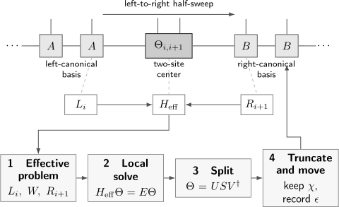
Anatomy of a left-to-right two-site DMRG step. Canonical tensors define orthonormal effective bases, the reusable environments define $H_{\mathrm{eff}}$, the center solves a local eigenproblem, and an SVD both truncates the bond and moves the center. The reverse half-sweep interchanges left and right.

One sweep is not a physical time evolution. Its direction and intermediate states are algorithmic. Only the converged represented state and properly evaluated observables have physical meaning.

Why the method is called density-matrix renormalization group

In the original block formulation, a system block was enlarged and then compressed. The retained block states were the eigenvectors of a reduced density matrix with the largest eigenvalues.

For a bipartite target state,

$$\lvert\psi\rangle = \sum_a s_a \lvert a_L\rangle \lvert a_R\rangle,$$

the reduced density matrix is

$$\rho_L = \sum_a s_a^2 \lvert a_L\rangle\langle a_L\rvert.$$

Keeping its largest eigenvalues is exactly Schmidt truncation. Modern finite-system DMRG written in MPS language performs the same optimal local compression through the SVD of the center tensor.

The historical name can otherwise mislead:

• DMRG is not a real-space renormalization-group flow that preserves every low-energy state.
• The density matrix belongs to the chosen target state or target ensemble.
• Modern implementations need not explicitly construct and diagonalize a dense reduced density matrix.
• The method is best understood as variational MPS optimization with adaptive Schmidt bases.

White introduced the density-matrix selection principle in 1992 and developed the finite-system algorithms in 1993. The later MPS interpretation made the variational state class and entanglement limitation explicit.

Why one-dimensional gapped systems are favorable

Three structures cooperate.

Local entanglement geometry

For a contiguous cut of an open one-dimensional chain, one MPS bond crosses the cut:

$$S_A \le \ln\chi.$$

Ground states of broad classes of local gapped one-dimensional Hamiltonians obey an area law. Their Schmidt spectra often decay sufficiently rapidly that moderate bond dimensions capture local observables and energies accurately.

The precise theorem status and converse cautions belong to Area Laws. An area law is not by itself a certificate that a particular $\chi$ is adequate or that a local optimizer will find the desired state.

Local Hamiltonian structure

Short-range one-dimensional Hamiltonians admit compact MPO representations. Their effective actions can be evaluated from left and right environments without constructing the full Hamiltonian matrix.

Reusable canonical bases

Canonical MPS gauges provide orthonormal effective block bases and stable local norm matrices. As the center moves, most contractions are reused rather than recomputed from scratch.

The favorable implication is therefore conditional:

$$\begin{gathered} \text{local 1D Hamiltonian} \\ + \text{compressible entanglement} \\ + \text{successful variational search} \\ \Longrightarrow \text{accurate DMRG} \\ \text{at accessible }\chi. \end{gathered}$$

Removing any one condition can change the conclusion.

Entanglement and geometry limitations

Critical states

A critical ground state has entanglement that grows with subsystem size. Finite bond dimension then creates an artificial correlation length $\xi_\chi$. A stable energy at one $\chi$ does not distinguish a physical gap from finite-entanglement saturation.

Critical studies require a controlled grid in system size and bond dimension, with the regimes in Entanglement and Criticality kept distinct.

Cylinders and two-dimensional lattices

Mapping a width-$W$ cylinder to a one-dimensional ordering makes a transverse cut intersect $O(W)$ physical bonds. If

$$S_{\mathrm{cut}} \sim \alpha W,$$

then an MPS needs at least

$$\chi \gtrsim e^{\alpha W}$$

to supply the corresponding Schmidt-rank capacity. DMRG can be powerful on cylinders, but cost generally grows rapidly with width. Width convergence, ordering, aspect ratio, boundary pinning, and sector selection all become part of the physical inference.

Volume-law states

Highly excited states, generic long-time states after global quenches, and other volume-law targets can require

$$\ln\chi \propto L$$

across central cuts. The required bond dimension is then exponential in system size.

Long-range couplings and large local spaces

Long-range Hamiltonians may need a larger MPO bond dimension or an approximation to the interaction kernel. Bosonic, molecular, or orbital problems may also need a large local basis. DMRG then carries both a bond truncation and a local-basis or operator-compression error.

Cost statements without false precision

For roughly uniform local dimension $q$, MPS bond dimension $\chi$, and MPO bond dimension $w$, the work per open-chain sweep is often:

• linear in chain length $L$;
• polynomial in $q$ and $w$;
• dominated by contractions with a cost commonly cubic in $\chi$.

But there is no universal formula such as “DMRG costs $L\chi^3$” without qualifications. The exponent and prefactor depend on:

• one-site versus two-site updates;
• contraction order;
• MPO structure and range;
• symmetry block sizes;
• local eigensolver iterations;
• target-state multiplicity;
• boundary conditions;
• memory strategy and parallelization.

A defensible scaling claim reports measured wall time and memory against $L$, $\chi$, $w$, and symmetry content for the actual calculation.

Symmetry, ordering, and boundaries

Symmetry sectors

Block-sparse tensors can enforce conserved charges such as particle number or total spin projection:

$$Q_{\mathrm{left}} + q_s = Q_{\mathrm{right}}.$$

This reduces cost and prevents drift out of the selected sector. It can also prevent the optimizer from reaching a lower state in another sector. A ground-state claim must compare all physically relevant sectors or justify the selected one.

For non-Abelian symmetries, multiplet structure changes the meaning of “number of kept states.” Reports should distinguish reduced multiplets from total bond-state dimension.

Site and orbital ordering

DMRG sees the one-dimensional order supplied to it. A poor ordering can turn short-range physical correlations into long-range MPS entanglement and enlarge the MPO. Ordering is therefore a variational design choice, not a cosmetic indexing convention.

Boundary conditions

Open boundaries align naturally with canonical MPS sweeps. They also create edge profiles and may select among nearly degenerate states. Periodic boundaries can reduce edge effects but are usually less favorable computationally.

Bulk observables should be measured in controlled central windows or extrapolated with boundary effects exposed. See Boundary Conditions on Lattices.

Initialization and metastability

Common initializations include:

• a product state in the desired sector;
• a random symmetry-compatible MPS;
• a converged state at smaller $\chi$;
• a nearby parameter point;
• an exact-diagonalization state on a smaller system;
• a state with deliberately chosen boundary pinning or unit cell.

Continuation can accelerate a scan, but it can also preserve hysteresis and metastability. Near first-order transitions, competing orders, topological sectors, or nearly degenerate manifolds, use independent initial states that favor different candidates.

Agreement after only one initialization is evidence about one optimization basin. It is not evidence that no lower basin exists.

A convergence hierarchy

Convergence should be established in layers.

Local-solver convergence

At every center, monitor:

$$r_{\mathrm{loc}} = \left\| H_{\mathrm{eff}}a - E_{\mathrm{loc}}a \right\|.$$

The local tolerance should be tighter than the physical changes one intends to resolve. Oversolving early sweeps can waste work because the environments are still changing; undersolving late sweeps can create false stationarity.

Sweep convergence

Across complete sweeps, track:

$$\Delta E_{\mathrm{sweep}} = \left| E^{(n)} - E^{(n-1)} \right|,$$

as well as changes in representative local observables, correlations, entanglement data, and symmetry labels.

The energy can converge before delicate observables. A small $\Delta E_{\mathrm{sweep}}$ only shows that the current trajectory has become stationary.

Bond convergence

Repeat the calculation over a sequence

$$\chi_1 < \chi_2 < \cdots$$

or over decreasing discarded-weight targets. Compare:

• energy and energy density;
• energy variance;
• local and long-distance observables;
• correlation lengths;
• Schmidt spectra and entropies;
• state quantum numbers;
• dependence on initialization and sweep schedule.

Hamiltonian variance

For a normalized state,

$$\sigma_H^2 = \langle H^2\rangle - \langle H\rangle^2$$

and equivalently

$$\sigma_H = \left\| (H-E)\lvert\psi\rangle \right\|.$$

An exact eigenstate has zero variance. Variance probes the full represented state rather than one local effective problem, making it stronger evidence than sweep stationarity alone.

Energy-versus-variance extrapolation can be useful near a well-isolated eigenstate, but linearity is not a theorem for arbitrary state families or fitting windows.

Size and geometry convergence

Only after controlling solver and bond errors should one infer:

$$\begin{gathered} L\to\infty, \\ W\to\infty, \\ \text{or another physical limit}. \end{gathered}$$

For critical systems, finite size and finite entanglement are competing infrared cutoffs. For cylinders, length, width, aspect ratio, and bond dimension are separate axes.

Error ledger

Error source	Control variable	Diagnostic	Unsupported shortcut
local eigensolve	residual tolerance, subspace size	$r_{\mathrm{loc}}$	one converged center proves a converged sweep
optimization basin	sweeps, restarts, initialization	independent histories and final energies	the first stationary state is the ground state
MPS representation	$\chi$ or truncation target	bond grid, Schmidt tails, variance, observables	a small discarded weight is a global error bar
symmetry sector	charge and multiplet labels	compare relevant sectors	the cheapest sector contains the ground state
local basis or MPO	local cutoff, operator compression	cutoff and MPO convergence	bond convergence controls every approximation
finite length	$L$, boundary condition	finite-size sequence	bulk-looking center data are thermodynamic
finite width	$W$, ordering, aspect ratio	width sequence and reordered checks	one cylinder represents a 2D phase
observable extraction	contraction and normalization	sum rules, independent evaluations	energy convergence implies correlation convergence

The total scientific claim is limited by the least controlled row.

Stopping logic

There is no universal energy threshold that makes DMRG converged. A defensible stopping rule is conjunctive:

$$\begin{gathered} r_{\mathrm{loc}} \text{ is small}, \\ \Delta E_{\mathrm{sweep}} \text{ is stable}, \\ \sigma_H \text{ meets the target}, \\ \text{observables} \\ \text{are sweep-stable}, \\ \text{larger }\chi \\ \text{changes no reported conclusion}, \\ \text{independent initializations} \\ \text{agree or are explained}. \end{gathered}$$

The tolerances should be chosen from the observable and claim, not copied from another model. A phase boundary, a tiny excitation gap, and a coarse ground-state energy require different evidence.

Ground-state reporting checklist

A reproducible DMRG result should state:

1. Hamiltonian convention, units, and parameter values.
2. Site or orbital ordering and local basis.
3. System length, width, aspect ratio, and boundary conditions.
4. Conserved symmetries and target sector.
5. MPS and MPO conventions relevant to the calculation.
6. One-site or two-site update and any enrichment or mixing.
7. Bond schedule or discarded-weight target.
8. Number and definition of sweeps.
9. Local eigensolver and residual tolerance.
10. Initialization set and continuation strategy.
11. Maximum and representative discarded weights.
12. Final energy variance and canonical residuals.
13. Bond, sweep, size, and width convergence data.
14. Observable windows, extrapolation forms, and uncertainty.
15. Exact, analytic, or independent-method benchmarks.

Reporting only the final bond dimension and energy is insufficient.

Benchmark logic

Product-state fixed point

For

$$H = - \sum_{i=1}^{L}Z_i,$$

the ground state is a product state with $\chi=1$. A DMRG implementation should recover:

$$E_0 = -L, \qquad \sigma_H^2 = 0, \qquad \epsilon_{\mathrm{disc}} = 0.$$

This checks local basis ordering, Hamiltonian signs, normalization, and the sweep loop. It does not test nontrivial entanglement.

Small-chain overlap window

For an interacting chain small enough for exact diagonalization, compare:

$$E_{\mathrm{DMRG}}, \qquad \sigma_H, \qquad \left| \langle\psi_{\mathrm{ED}} \vert \psi_{\mathrm{DMRG}}\rangle \right|^2,$$

along with several observables. Energy agreement alone can conceal an incorrect vector inside a nearly degenerate subspace.

Heisenberg-chain sequence

For the antiferromagnetic spin-$1/2$ chain,

$$H = J \sum_{i} \mathbf S_i\cdot\mathbf S_{i+1}, \qquad J>0,$$

use small-$L$ exact diagonalization, then increase $L$ and $\chi$. The infinite-chain energy density is a valuable analytic check, but open-boundary finite systems contain edge and finite-size corrections. The canonical Heisenberg Model page fixes the model conventions and physical interpretation.

Excited states and other extensions

The cleanest excited-state target is often the lowest state in a different exact symmetry sector. Within one sector, common strategies include:

• explicit orthogonality constraints against lower states;
• projector penalties;
• state-averaged reduced density matrices;
• block or multi-state optimization;
• tangent-space or correction-vector methods for specific responses.

A projector-penalty target has the schematic form

$$H' = H + \sum_{n<k} \mu_n \lvert\psi_n\rangle\langle\psi_n\rvert.$$

The penalty strengths, orthogonality errors, and accumulated errors in the lower states must be controlled. An excited-state variational search can converge to the wrong root even when its local residuals are small.

Infinite-system algorithms, dynamical DMRG, finite-temperature purification, and non-Hermitian transfer problems share tensor-network ingredients but have distinct fixed points and validation requirements. They should not be inferred from finite ground-state DMRG without a dedicated analysis.

Common mistakes

Calling MPS and DMRG the same object

MPS is a state representation. DMRG is an optimization family acting on that representation.

Treating the final sweep change as an error bar

A small energy change measures stationarity of one trajectory. It does not bound bond, sector, basis, or finite-size error.

Interpreting discarded weight globally

Discarded weight belongs to a specified local truncation. Its impact depends on all later updates and on the observable.

Assuming two-site DMRG is strictly monotone

The local solve is variational before truncation. The SVD minimizes state-norm error, not post-truncation energy.

Assuming one-site DMRG can always change the bond basis

A fixed bond space can trap the optimizer. Enrichment or a two-site warm-up may be needed.

Mixing numerical and physical gaps

The local effective-Hamiltonian gap, the MPS transfer gap, and the physical excitation gap are different objects.

Hiding the ordering

For ladders, cylinders, orbitals, or fermions, ordering changes entanglement, MPO range, and signs.

Comparing only energies across candidate phases

Near-degenerate variational states can have almost identical energies and different correlations, entanglement, or symmetry structure.

Extrapolating before controlling bond error

A finite-size fit through bond-limited data can manufacture a stable but incorrect thermodynamic trend.

Exercises

Exercise 1: Derive the local effective problem

Let $\lvert\psi(a)\rangle=Xa$ with

$$H_{\mathrm{eff}} = X^\dagger H X, \qquad N_{\mathrm{eff}} = X^\dagger X.$$

Derive the stationary equation for the local Rayleigh quotient. Explain why mixed-canonical form changes a generalized eigenproblem into an ordinary one.

Solution

Write

$$\mathcal E(a) = \frac{ a^\dagger H_{\mathrm{eff}}a }{ a^\dagger N_{\mathrm{eff}}a }.$$

Stationarity with respect to $a^\dagger$ gives

$$H_{\mathrm{eff}}a - \mathcal E(a) N_{\mathrm{eff}}a = 0.$$

Thus

$$H_{\mathrm{eff}}a = E_{\mathrm{loc}} N_{\mathrm{eff}}a.$$

In mixed-canonical form the effective left and right bases are orthonormal. Therefore $X^\dagger X=I$, so

$$H_{\mathrm{eff}}a = E_{\mathrm{loc}}a.$$

If a code in canonical gauge produces a badly conditioned $N_{\mathrm{eff}}$, its canonicalization or environment contractions should be audited.

Exercise 2: Read a two-site truncation

A normalized two-site center has Schmidt probabilities

$$\begin{gathered} (p_1,p_2,p_3) = (0.49,0.36,0.10), \\ (p_4,p_5) = (0.04,0.01). \end{gathered}$$

If only $\chi=2$ values are kept, find the discarded weight, retained norm, normalized-state fidelity, and the single-truncation worst-case observable bound.

Solution

The discarded weight is

$$\epsilon_{\mathrm{disc}} = 0.10+0.04+0.01 = 0.15.$$

The unnormalized retained state has norm squared

$$1-\epsilon_{\mathrm{disc}} = 0.85.$$

Its norm is therefore

$$\sqrt{0.85} \approx 0.922.$$

After normalization, its squared overlap with the original state is

$$F = \left| \langle\psi\vert\psi_\chi\rangle \right|^2 = 0.85.$$

For a bounded observable,

$$\begin{aligned} \left| \langle O\rangle_\psi - \langle O\rangle_{\psi_\chi} \right| &\le 2\sqrt{0.15} \lVert O\rVert_\infty \\ &\approx 0.775 \lVert O\rVert_\infty. \end{aligned}$$

This deliberately loose bound concerns one truncation. It is not a global sweep error estimate.

Exercise 3: Audit monotonicity

Classify each statement as correct or incorrect.

1. An exactly solved one-site update in exact canonical gauge cannot increase the variational energy.
2. An exactly solved two-site update cannot increase the energy after SVD truncation.
3. The global optimum cannot increase when every allowed bond dimension is enlarged.
4. A practical run at larger $\chi$ must always return a lower energy.

Solution

Statement 1 is correct under its assumptions. The previous center tensor belongs to the local search space, so exact minimization cannot do worse.

Statement 2 is incorrect. The pre-truncation local state is variationally improved, but the SVD selects the best state-norm truncation rather than the minimum-energy state at the retained rank.

Statement 3 is correct. Enlarging all bond bounds nests the variational classes, so their exact global minima are monotone.

Statement 4 is incorrect. A practical nonlinear optimization can land in a worse basin, use a looser local tolerance, or target a different effective sector. The variational-class statement does not guarantee algorithmic success.

Exercise 4: Separate local and global residuals

A run reports

$$r_{\mathrm{loc}} < 10^{-11}$$

at every center but has

$$\sigma_H = 10^{-3}.$$

What has converged, and what has not?

Solution

Every recorded center tensor accurately solves its current effective eigenproblem. The nonzero global variance shows that the final MPS is not comparably close to an exact eigenstate of the full Hamiltonian.

Possible causes include:

• inadequate bond dimension;
• a sweep that has not reached a fixed point;
• inconsistent or stale environments;
• truncation after accurate local solves;
• convergence to a variationally stationary but imperfect state.

The local residual and global variance answer different questions. The stronger ground-state claim must wait for bond and sweep studies and for the variance to meet the physical target.

Exercise 5: Design a critical-chain study

Explain why the grid

$$L \in \{64,128,256\}, \qquad \chi = 128$$

cannot by itself establish critical finite-size scaling. Propose a better design.

Solution

At fixed $\chi$, the MPS has an induced finite-entanglement scale $\xi_\chi$. If $L$ exceeds or approaches this scale, apparent saturation can mimic a physical gap or distort critical exponents.

A better study uses a two-dimensional grid:

$$\begin{gathered} L \in \{64,128,256,\ldots\}, \\ \chi \in \{128,256,512,\ldots\}. \end{gathered}$$

For each $L$, verify that energies, correlations, entropies, and fitted quantities are stable as $\chi$ increases, or perform an explicit joint finite-size and finite-entanglement analysis. The study should also vary boundaries or central fitting windows and check symmetry and initialization dependence.

Exercise 6: Build a ground-state evidence package

A two-site calculation on a width-six cylinder reports a stable energy after twelve sweeps at $\chi=4000$. List the minimum additional evidence needed before calling the state the two-dimensional ground-state phase.

Solution

At minimum, require:

• local residuals and the final global energy variance;
• energy, observables, entanglement, and correlations over a sequence of $\chi$;
• discarded-weight profiles rather than one maximum value;
• independent initial states favoring plausible competing phases;
• explicit symmetry and topological-sector labels;
• length and aspect-ratio convergence at fixed width;
• several widths, with controlled boundary conditions and ordering;
• central-window and edge-sensitivity checks;
• small-system exact or cross-method benchmarks where possible;
• stability of the phase diagnostic, not merely the energy.

A width-six cylinder is a quasi-one-dimensional finite geometry. Calling its state a two-dimensional phase requires a width extrapolation or a carefully qualified evidence horizon.

Summary

Finite-system DMRG minimizes the energy over an MPS class by moving a one-site or two-site variational center through the chain. Canonical gauges make the local norm matrix the identity, and contracted environments define a matrix-free effective Hamiltonian:

$$H_{\mathrm{eff}}a = E_{\mathrm{loc}}a.$$

One-site updates are fixed-bond and strictly variational under controlled assumptions. Two-site updates adapt the bond basis, then use an SVD with local discarded weight

$$\epsilon_{\mathrm{disc}} = \sum_{a>\chi}s_a^2.$$

The method is favorable when one-dimensional Hamiltonian structure, compressible ground-state entanglement, and a successful optimization basin coincide. Criticality, cylinder width, volume-law entanglement, long-range operators, large local bases, and competing sectors can all defeat that favorable regime.

No single diagnostic certifies a DMRG result. A mature claim combines local residuals, complete-sweep stability, energy variance, bond convergence, initialization tests, symmetry checks, observable convergence, finite-size or width control, and independent benchmarks.

References

1. S. R. White, “Density Matrix Formulation for Quantum Renormalization Groups,” Physical Review Letters 69, 2863–2866 (1992), doi:10.1103/PhysRevLett.69.2863.
2. S. R. White, “Density-Matrix Algorithms for Quantum Renormalization Groups,” Physical Review B 48, 10345–10356 (1993), doi:10.1103/PhysRevB.48.10345.
3. S. Östlund and S. Rommer, “Thermodynamic Limit of Density Matrix Renormalization,” Physical Review Letters 75, 3537–3540 (1995), doi:10.1103/PhysRevLett.75.3537.
4. S. Rommer and S. Östlund, “Class of Ansatz Wave Functions for One-Dimensional Spin Systems and Their Relation to the Density Matrix Renormalization Group,” Physical Review B 55, 2164–2181 (1997), doi:10.1103/PhysRevB.55.2164.
5. U. Schollwöck, “The Density-Matrix Renormalization Group,” Reviews of Modern Physics 77, 259–315 (2005), doi:10.1103/RevModPhys.77.259.
6. I. P. McCulloch, “From Density-Matrix Renormalization Group to Matrix Product States,” Journal of Statistical Mechanics: Theory and Experiment (2007) P10014, doi:10.1088/1742-5468/2007/10/P10014.
7. M. B. Hastings, “An Area Law for One-Dimensional Quantum Systems,” Journal of Statistical Mechanics: Theory and Experiment (2007) P08024, doi:10.1088/1742-5468/2007/08/P08024.
8. F. Verstraete, V. Murg, and J. I. Cirac, “Matrix Product States, Projected Entangled Pair States, and Variational Renormalization Group Methods for Quantum Spin Systems,” Advances in Physics 57, 143–224 (2008), doi:10.1080/14789940801912366.
9. N. Schuch, M. M. Wolf, F. Verstraete, and J. I. Cirac, “Entropy Scaling and Simulability by Matrix Product States,” Physical Review Letters 100, 030504 (2008), doi:10.1103/PhysRevLett.100.030504.
10. U. Schollwöck, “The Density-Matrix Renormalization Group in the Age of Matrix Product States,” Annals of Physics 326, 96–192 (2011), doi:10.1016/j.aop.2010.09.012.
11. G. K.-L. Chan and S. Sharma, “The Density Matrix Renormalization Group in Quantum Chemistry,” Annual Review of Physical Chemistry 62, 465–481 (2011), doi:10.1146/annurev-physchem-032210-103338.
12. E. M. Stoudenmire and S. R. White, “Studying Two-Dimensional Systems with the Density Matrix Renormalization Group,” Annual Review of Condensed Matter Physics 3, 111–128 (2012), doi:10.1146/annurev-conmatphys-020911-125018.
13. C. Hubig, I. P. McCulloch, U. Schollwöck, and F. A. Wolf, “Strictly Single-Site DMRG Algorithm with Subspace Expansion,” Physical Review B 91, 155115 (2015), doi:10.1103/PhysRevB.91.155115.
14. Ö. Legeza and J. Sólyom, “Optimizing the Density-Matrix Renormalization Group Method Using Quantum Information Entropy,” Physical Review B 68, 195116 (2003), doi:10.1103/PhysRevB.68.195116.

Further study

• Tensor Networks: Computational Guide
• Matrix Product States Preview
• Entanglement Spectrum
• Area Laws
• Entanglement and Criticality
• Variational Many-Body States
• Lanczos Method Preview
• Symmetry Sectors in Many-Body Numerics
• Finite-Size Scaling in Numerics
• Exact Diagonalization Preview
• Validation Tests
• Computational Quantum Mechanics Roadmap