Computational Many-Body Overview

A many-body computation is a structured argument, not merely a number produced by a solver. The argument begins with a Hamiltonian, state or ensemble, observable, boundary condition, and physical limit. It then chooses a representation and method whose assumptions match the problem, establishes numerical control, and only afterward makes a physical claim.

The central distinction is

$$\begin{gathered} \text{computed object} \neq \text{physical conclusion}, \\ \text{computed object} + \text{validation} \\ + \text{limit control} \\ \Longrightarrow \text{qualified conclusion}. \end{gathered}$$

This distinction matters especially in many-body quantum mechanics. A finite matrix can be diagonalized to machine precision while remaining a poor approximation to the thermodynamic system. A Monte Carlo estimate can have a tiny reported standard error while still being biased by equilibration or an unresolved sign problem. A variational state can have a stable energy while missing the correlations needed for the observable of interest.

Purpose and Canonical Scope

This page owns the many-body logic for selecting and interpreting computational methods. It explains:

• how the physical question determines the computational target;
• which structures make an exponentially large Hilbert space tractable;
• how exact diagonalization, Krylov methods, quantum Monte Carlo, and tensor networks answer different questions;
• how residuals, variances, sum rules, exact limits, and cross-method comparisons validate a result;
• how finite-size, truncation, statistical, and solver errors remain distinct;
• what evidence is needed before a finite calculation supports a thermodynamic claim;
• how to report a calculation so another researcher can reproduce and audit it.

This is a bridge chapter. Detailed algorithms, data structures, software architecture, convergence proofs, production implementations, and performance engineering belong in the future Computational QM volume. The Computational Quantum Mechanics Roadmap gives the broad learning route, Math Needed for Computational QM owns the numerical prerequisites, and Computational QM References is the general reading guide.

Within the present volume:

• Scaling of Hilbert Space owns basis-size counts and their asymptotics.
• Exact Diagonalization Preview owns finite basis construction, sparse Hamiltonian action, complete versus targeted eigensystems, and finite-system observables.
• Thermodynamic Limit owns the physical meaning and order of large-system limits.
• Tensor Networks Preview owns the conceptual tensor-network language.
• Matrix Product States Preview owns MPS canonical forms, transfer operators, and one-dimensional entanglement structure.
• Tensor Networks: Computational Guide owns network-family routing, convergence designs, stopping criteria, and reporting standards for finite-bond calculations.
• DMRG Preview owns finite-system effective eigenproblems, one-site and two-site sweeps, truncation, and ground-state convergence.
• Dynamical Correlation Functions Numerically owns the comparison of Lehmann, continued-fraction, and real-time routes, including matched resolution kernels and cross-method validation.
• Benchmark Problems owns the reproducible MB-Bxxx suite for finite clusters, ideal gases, the BCS gap equation, and Ising-gap scaling.
• Reproducible Notebooks owns the status-aware many-body notebook inventory, canonical filenames, and admission gates.
• Spectral Functions owns the exact spectral definitions and sum rules used by numerical calculations.
• Boundaries with Neighboring Subjects owns the formal division between many-body physics and reusable computational infrastructure.

Here these ingredients are assembled into a decision and evidence framework without duplicating their canonical derivations.

Declare the Physical Question First

A reproducible calculation starts from a problem declaration such as

$$\mathcal P = \left( H, \mathcal S, \mathcal B, \rho, O, \mathcal L, \varepsilon_{\mathrm{target}} \right).$$

The entries record:

• the Hamiltonian $H$ and all parameter conventions;
• the symmetry sector or constrained space $\mathcal S$;
• geometry and boundary conditions $\mathcal B$;
• the state or ensemble $\rho$;
• the target observable $O$;
• the physical limit $\mathcal L$ to be inferred;
• the requested accuracy or resolution $\varepsilon_{\mathrm{target}}$.

For example, “find the ground-state energy” is incomplete. One must still say whether the system is a finite open chain or a periodic lattice, whether particle number is fixed, which symmetry sector contains the target state, whether the reported quantity is total energy or energy density, and whether the objective is a finite-size benchmark or a thermodynamic extrapolation.

The observable should be declared before the method. Ground-state energy, a small excitation gap, a long-distance correlator, an entanglement spectrum, a finite-temperature susceptibility, and a real-time spectral function can demand very different representations even for the same $H$.

A useful claim template

Write the intended claim before running the calculation:

For the stated model, geometry, sector, and parameter range, observable $O_L$ converges under the declared numerical controls; the sequence of controlled finite systems is consistent with the stated large-system behavior.

This wording separates three questions:

1. Was the finite problem solved correctly?
2. Is the sequence of finite problems controlled?
3. Does the sequence support the proposed physical interpretation?

No single solver tolerance answers all three.

Why Structure Matters More Than Raw Dimension

For a local Hilbert-space dimension $q$ on $L$ sites, an unconstrained product basis has dimension $q^L$. Fixed-particle sectors produce binomial or multinomial dimensions, but their largest sectors still grow exponentially. The exact counts and asymptotics belong to Scaling of Hilbert Space.

The practical question is therefore not only

$$D = \dim\mathcal H,$$

but also:

$$\begin{gathered} \text{sparsity of }H \\ \text{exact symmetries} \\ \text{target-state entanglement} \\ \text{sign or phase of weights} \\ \text{spectral region required} \\ \text{effective geometry} \end{gathered}$$

Several forms of structure can replace an impossible generic problem with a tractable special one:

• Locality makes Hamiltonian application sparse or factorizable.
• Symmetry restricts the calculation to invariant sectors.
• Spectral targeting avoids computing eigenvectors that are never used.
• Low entanglement permits compressed tensor-network representations.
• Positive statistical weights permit efficient stochastic sampling in favorable models.
• Translation invariance can reduce both basis size and observable noise.
• Exactly solvable limits and sum rules supply strong validation targets.

These structures are method-dependent resources. Sparsity helps Krylov methods but does not by itself guarantee easy real-time evolution. An area law helps matrix-product-state methods, but not if the chosen ordering converts short-range interactions into highly nonlocal ones. A formally valid path integral does not imply a useful Monte Carlo distribution if its weights fluctuate in sign or phase.

The Evidence Pipeline

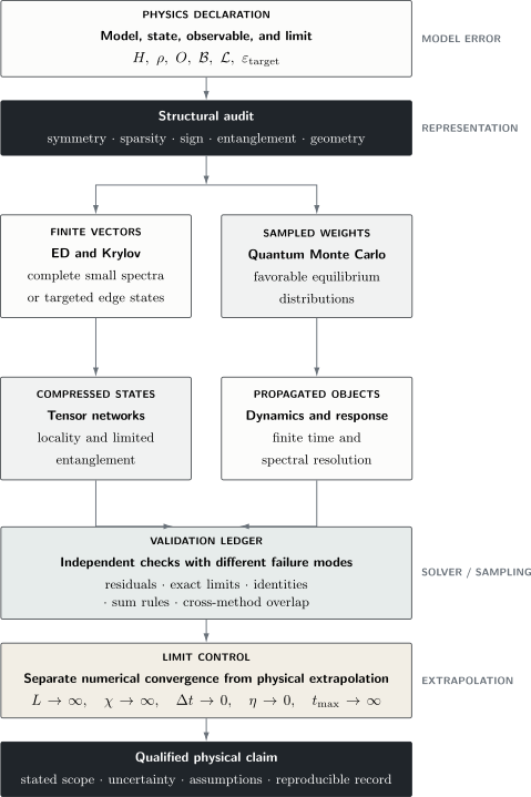
A trustworthy numerical claim preserves the entire chain from the physical declaration to the inferred limit. The four side labels identify distinct places where uncertainty enters; tightening a solver tolerance does not remove a model, representation, or extrapolation error.

The pipeline is deliberately directional. Method choice occurs only after the target and exploitable structure are known. Validation precedes extrapolation. A polished thermodynamic plot cannot repair a finite-system calculation that failed its residual, sum-rule, equilibration, or truncation checks.

Representation Comes Before Algorithm

The same many-body problem can be represented in several inequivalent computational forms.

Basis-state representation

Occupation strings, spin configurations, momentum occupations, or symmetry-adapted combinations produce vectors

$$|\psi\rangle = \sum_{a=1}^{D} c_a|a\rangle.$$

This representation is natural for exact diagonalization and Krylov methods. Its decisive costs are storing vectors of length $D$, applying $H$ efficiently, and identifying the correct sectors. Constructing a dense $D\times D$ matrix is usually unnecessary when only the action $v\mapsto Hv$ is needed.

Sampled configuration representation

A partition function or expectation value may be rewritten as

$$\begin{aligned} Z &= \sum_C W(C), \\ \langle O\rangle &= \frac{ \sum_C W(C)O(C) }{ \sum_C W(C) }. \end{aligned}$$

When $W(C)\geq0$ and can be sampled, stochastic methods can avoid enumerating every configuration. The representation shifts the challenge from vector storage to autocorrelation, equilibration, estimator variance, and possible sign or phase cancellations.

Compressed tensor representation

A one-dimensional state may be written schematically as

$$|\psi\rangle = \sum_{\{s_i\}} A_1^{s_1} A_2^{s_2} \cdots A_L^{s_L} |s_1s_2\cdots s_L\rangle.$$

The internal bond dimensions control expressive capacity. This does not defeat exponential complexity for arbitrary states. It exploits the fact that many physically important low-energy states of local one-dimensional systems occupy a highly structured corner of Hilbert space. The conceptual foundations are developed in Matrix Product States Preview.

Propagated state or operator representation

Dynamics may target

$$|\psi(t)\rangle = e^{-iHt/\hbar} |\psi(0)\rangle$$

without diagonalizing $H$. Krylov propagation, product formulas, tensor-network time evolution, and stochastic real-time methods have different failure modes. The required maximum time, conservation laws, entanglement growth, and desired frequency resolution should be declared before choosing among them.

Method Families at a Glance

• Complete spectrum of a modest symmetry sector. Exact diagonalization is the natural first route; require residuals, orthogonality, trace identities, and exact-limit checks.
• A few spectral-edge states with sparse $H$ action. Start with Lanczos or another Krylov eigensolver; control near-degeneracy, orthogonality, residuals, and restarts.
• Equilibrium averages with nonnegative or mild-sign weights. Quantum Monte Carlo is a candidate; establish equilibration, autocorrelation, $N_{\mathrm{eff}}$, and agreement among independent runs.
• A one-dimensional low-entanglement ground state. MPS and DMRG are natural; vary bond dimension and initialization while monitoring variance and discarded weight.
• Short- or intermediate-time local dynamics. Krylov or tensor-network propagation can exploit locality; test the step size, conservation laws, entanglement growth, and reachable time.
• Response in an accessible spectral window. Lehmann, Krylov, correction-vector, or time-domain methods may apply; check sum rules, finite-size poles, broadening, and resolution.

“Natural” does not mean universally best. A two-dimensional frustrated magnet can be small enough for exact diagonalization, sign-problematic for quantum Monte Carlo, and difficult for tensor networks. A one-dimensional model at long real times can outgrow an initially efficient MPS description because entanglement increases rapidly. Method selection is a statement about the target regime, not a permanent label attached to the Hamiltonian.

Exact Diagonalization and Krylov Thinking

Exact diagonalization solves a finite, represented eigenproblem. It is exact only relative to:

• the chosen finite geometry;
• the chosen basis or local cutoff;
• the selected symmetry sector;
• floating-point arithmetic and eigensolver tolerances.

If the complete finite spectrum is not needed, a Krylov space

$$\begin{gathered} \mathcal K_m \left( H,|v\rangle \right) \\ = \operatorname{span} \left\{ \begin{array}{c} |v\rangle, H|v\rangle, \ldots, \\ H^{m-1}|v\rangle \end{array} \right\} \end{gathered}$$

can target extremal eigenpairs or matrix functions while storing far fewer vectors than the full Hilbert-space dimension. Lanczos Method Preview develops the many-body ground-state and response workflow; Sparse Eigensolvers retains the general numerical recurrence and solver engineering.

Residuals are local certificates

For a normalized approximate eigenvector $|\widetilde\psi\rangle$ and approximate eigenvalue $\widetilde E$, define

$$|r\rangle = \left( H-\widetilde E \right) |\widetilde\psi\rangle.$$

For a finite Hermitian $H$,

$$\operatorname{dist} \left( \widetilde E, \operatorname{spec}H \right) \leq \lVert r\rVert.$$

Thus a small residual certifies proximity to some eigenvalue. It does not by itself identify the state, resolve a near-degenerate multiplet, or establish that the basis and finite geometry represent the desired physics.

If

$$\widetilde E = \langle\widetilde\psi| H |\widetilde\psi\rangle,$$

then

$$\lVert r\rVert^2 = \langle H^2\rangle - \langle H\rangle^2 \equiv \sigma_H^2.$$

Energy variance is therefore both an eigenstate diagnostic and a useful cross-method quantity. A low energy with a visibly nonzero variance is not yet a converged eigenstate.

Variational control is specific

For a normalized trial state and a Hermitian Hamiltonian bounded below,

$$E_{\mathrm{var}} = \langle\psi_{\mathrm{var}}| H |\psi_{\mathrm{var}}\rangle \geq E_0.$$

The upper bound concerns the ground-state energy. It does not automatically bound an order parameter, correlation length, excitation gap, or real-time observable. Those quantities require their own convergence evidence.

Stochastic Thinking

Suppose correlated samples $O_1,\ldots,O_N$ estimate an equilibrium mean. With one common convention for the integrated autocorrelation time,

$$\tau_{\mathrm{int}} = \frac12 + \sum_{t=1}^{\infty} \rho_O(t),$$

the effective sample size is approximately

$$N_{\mathrm{eff}} \simeq \frac{N} {2\tau_{\mathrm{int}}}.$$

The standard error then scales as

$$\operatorname{SE} \left( \overline O \right) \simeq \sqrt{ \frac{\operatorname{Var}(O)} {N_{\mathrm{eff}}} }.$$

The convention for $\tau_{\mathrm{int}}$ must be stated because factors of two vary across communities. More importantly, this estimate assumes the chain has equilibrated and that the autocorrelation analysis reaches the slowest relevant mode.

If weights have signs or phases, write

$$W(C) = |W(C)|s(C),$$

so that

$$\langle O\rangle_W = \frac{ \langle sO\rangle_{|W|} }{ \langle s\rangle_{|W|} }.$$

When the average sign becomes exponentially small, relative errors grow correspondingly and feasible system sizes or inverse temperatures can collapse. This is a structural obstruction, not merely a need for a longer run. Sign Problem Preview develops the many-body meaning, basis dependence, sign-free cases, and the precise scope of the generic complexity obstruction.

Tensor-Network Thinking

Across a bipartition, write a normalized pure state in Schmidt form:

$$|\psi\rangle = \sum_{\alpha} s_\alpha |\alpha\rangle_A |\alpha\rangle_B, \qquad \sum_\alpha s_\alpha^2 = 1.$$

Keeping the largest $\chi$ Schmidt values leaves discarded weight

$$\epsilon_{\mathrm{disc}} = \sum_{\alpha>\chi} s_\alpha^2.$$

This quantity is useful but not a universal error bar on every observable. Small discarded weight at each local truncation does not by itself prove that a sweep found the global variational optimum, that boundary effects are negligible, or that a long-distance correlator has converged.

A trustworthy tensor-network calculation therefore varies more than one control:

$$\begin{gathered} \chi, \qquad \text{sweep count}, \\ \text{initial state}, \qquad L, \\ \text{boundary condition}. \end{gathered}$$

Energy variance, symmetry quantum numbers, entanglement profiles, and agreement between independent initializations are complementary diagnostics. Near criticality, the required bond dimension can grow because the entanglement spectrum decays more slowly. During a global quench, entanglement growth can impose a reachable-time horizon even when short-time observables look well converged.

Four Error Classes That Must Not Be Collapsed

A useful audit keeps a vector of error sources:

$$\boldsymbol\varepsilon = \left( \varepsilon_{\mathrm{model}}, \varepsilon_{\mathrm{representation}}, \varepsilon_{\mathrm{solver}}, \varepsilon_{\mathrm{limit}} \right).$$

Model and physical-approximation error

This includes omitted interactions, an approximate effective Hamiltonian, a mean-field closure, uncertain parameters, or a mismatch between the model and the physical system. More digits from the same model do not reduce this error.

Representation error

Examples include a finite local occupation cutoff, momentum or real-space discretization, tensor-network bond dimension, Trotter decomposition, finite imaginary-time grid, or spectral broadening. Representation error can remain even when the algebraic solver is perfectly converged.

Solver or sampling error

This includes eigensolver residuals, incomplete optimization, time-step integration error, roundoff, Monte Carlo standard error, autocorrelation, and equilibration bias. These are the errors most directly controlled by numerical parameters, but they are only one part of the claim.

Limit and interpretation error

Finite-size extrapolation, continuum extrapolation, zero-temperature inference, infinite-time inference, and analytic continuation belong here. Choosing an unjustified fit form is not a solver error. Neither is mistaking a finite-size crossover for a phase transition.

It is often misleading to add these four entries into one scalar uncertainty. Some are statistical, some are deterministic bounds, some are fit-systematic ranges, and some are modeling assumptions. Report them separately, with the evidence supporting each estimate.

A Convergence Matrix

Changing one parameter at a time can hide coupled errors. Instead, think of a result as

$$O = O \left( L, \chi, \Delta\tau, m, N_{\mathrm{MC}}, \eta, t_{\max}, \ldots \right).$$

Here $L$ is system size, $\chi$ a bond dimension, $\Delta\tau$ an imaginary- or real-time step, $m$ a Krylov dimension, $N_{\mathrm{MC}}$ a sample count, $\eta$ a spectral broadening, and $t_{\max}$ a maximum propagation time.

A convergence matrix tests the parameters that can interact:

• Sector dimension or local cutoff. Energies and local observables should stabilize; the required cutoff can grow with interaction strength or density.
• Krylov dimension and residual tolerance. Target eigenpairs or propagated states should stabilize; near-degeneracy and long propagation times can demand larger spaces.
• Bond dimension. Energy, variance, correlations, and entropy should stabilize together; the required $\chi$ grows with size, criticality, and time.
• Monte Carlo length. Means and uncertainty estimates should stabilize; autocorrelation commonly grows near criticality.
• Time step. Conserved quantities and trajectories should stabilize; a smaller step does not cure an insufficient bond dimension.
• Broadening and maximum time. Spectral features should remain interpretable as $\eta$, $t_{\max}$, and finite-size level spacing are varied together.
• System size and geometry. Intensive observables and scaling combinations should stabilize; aspect ratio and boundary conditions can change the leading corrections.

The goal is not to make every parameter enormous. It is to identify a window where the target observable is insensitive to numerical controls at the precision required for the physical conclusion.

Finite Systems and Thermodynamic Claims

A numerical solver returns information about a declared finite representation. Before extrapolating it, use Finite-Size Effects to identify whether boundaries, quantized modes, shells, commensurability, correlation cutoffs, or finite-time resolution control the observable. The Thermodynamic Limit owns the target sequence.

There is no universal correction law: exponential, algebraic, logarithmic, oscillatory, and scaling-function behavior can each be appropriate under different hypotheses. Critical Exponents and Scaling owns critical scaling theory; Finite-Size Scaling in Numerics owns fit forms, covariance, omitted-size tests, competing models, data collapse, and uncertainty. A smooth trend or attractive collapse is not a substitute for that evidence chain.

Dynamical Correlations and Numerical Resolution

For a finite system, an exact spectral function is a sum of discrete lines. A common visualization replaces each delta function by a Lorentzian:

$$\delta(\omega-\omega_n) \longrightarrow \frac{1}{\pi} \frac{\eta} {(\omega-\omega_n)^2+\eta^2}.$$

The broadening $\eta$ is a numerical or presentation parameter unless a physical decay mechanism has been derived. A smooth curve at finite $L$ is therefore not automatically a continuum spectrum.

Time-domain methods introduce a related resolution scale:

$$\Delta\omega \gtrsim \frac{2\pi} {t_{\max}}.$$

Window functions, finite-time truncation, finite-size recurrences, and entanglement-limited propagation all affect line shapes. A dynamical calculation should report $t_{\max}$, time step, window, broadening or reconstruction method, and relevant sum rules. Spectral Functions provides the canonical definitions against which those outputs should be checked.

Dynamical Correlation Functions Numerically turns this compact warning into a method-selection and evidence workflow for direct Lehmann sums, Lanczos continued fractions, real-time Fourier transforms, and controlled broadening.

Worked Strategy: A Finite Spin Chain

Consider the periodic transverse-field Ising chain

$$\begin{gathered} \begin{aligned} H &= -J \sum_{i=1}^{L} \sigma_i^z \sigma_{i+1}^z \\ &\quad - h \sum_{i=1}^{L} \sigma_i^x, \end{aligned} \\ \sigma_{L+1}^z = \sigma_1^z. \end{gathered}$$

Transverse-Field Ising Model owns the model, its phases, and its analytic structure. Here it serves only as a computational decision example.

Suppose the target is the finite-size gap and evidence for ordering as $L$ grows.

Step 1: Declare sectors and observables

The global spin-flip operator

$$P = \prod_{i=1}^{L} \sigma_i^x$$

commutes with $H$. Translation also commutes with $H$ for periodic boundaries. The target gap must specify whether it is:

• the lowest excitation in the ground-state symmetry sector;
• the difference between opposite-parity ground states;
• the lowest excitation at a specified momentum.

These quantities need not have the same finite-size behavior.

For a finite symmetry eigenstate,

$$\langle M_z\rangle = 0, \qquad M_z = \frac{1}{L} \sum_i\sigma_i^z,$$

even where the thermodynamic system orders. A suitable finite-size diagnostic is

$$\langle M_z^2\rangle = \frac{1}{L^2} \sum_{i,j} \langle \sigma_i^z\sigma_j^z \rangle,$$

or the corresponding structure factor. Measuring only $\langle M_z\rangle$ would confuse exact finite-size symmetry with absence of thermodynamic order.

Step 2: Match the method to size and target

For small symmetry sectors, full diagonalization supplies the complete spectrum and trace identities. For larger sectors, a Lanczos calculation can target the lowest state in each relevant parity and momentum sector without storing every eigenvector. An MPS calculation can reach much longer one-dimensional chains, but then bond-dimension, initialization, and boundary-condition studies replace full-spectrum checks.

Step 3: Build a benchmark ladder

The evidence can be ordered from cheapest to strongest:

1. verify Hermiticity and the commutators with implemented symmetry operators;
2. compare $J=0$ and $h=0$ limits against direct product-state results;
3. check residuals and orthogonality of targeted eigenstates;
4. compare full diagonalization and Lanczos where both are feasible;
5. compare Lanczos and MPS energies and correlators on overlapping sizes;
6. vary $L$, sector, and boundary conditions before extrapolating.

Agreement on one energy is weaker than agreement on energy, gap, correlations, symmetry labels, and variance. Cross-method comparison is most informative when the two methods have different failure modes.

The many-body benchmark suite turns this ladder into nine fixed contracts with trusted spectra, observables, thermodynamic roots, and a boundary-corrected scaling sequence.

Step 4: Phrase the conclusion at the supported level

There is a hierarchy:

$$\begin{gathered} 1: \quad \text{finite-system fact} \\ 2: \quad \text{controlled size trend} \\ 3: \quad \text{thermodynamic inference} \\ 4: \quad \text{universality or external claim} \end{gathered}$$

Each level requires additional assumptions. A Level 1 residual cannot certify a Level 3 phase transition. A Level 3 model result does not by itself establish a Level 4 claim about a material.

Choosing a Method by the Obstruction

Method selection is often clearest when framed by what prevents a direct calculation.

• Only spectral-edge states matter, but the vector space is too large. Exploit sparsity with a Krylov or Lanczos route; guard against near-degeneracy and loss of orthogonality.
• The configuration sum is enormous, but its weights are nonnegative. Exploit importance sampling with quantum Monte Carlo; establish equilibration and autocorrelation control.
• A one-dimensional state has limited entanglement. Exploit Schmidt compression with MPS or DMRG; test bond and metastability convergence.
• A real-time state is manageable only briefly. Exploit locality with Krylov or tensor-network propagation; state the finite-time and entanglement horizon.
• A thermodynamic claim rests on small clusters. Exploit scaling and universality; expose uncertainty from corrections, shape, and boundary conditions.
• Several methods are individually fragile. Use an overlap window for a cross-method benchmark; remember that shared model and convention errors can survive agreement.

There is no universal ranking in which one family is more exact than another. Exactness is conditional:

• exact diagonalization is exact for a declared finite represented problem;
• Krylov results are controlled by residuals and subspace convergence;
• a variational method provides specific bounds and systematic families of trial states;
• Monte Carlo can be statistically unbiased for a declared representation while still suffering equilibration or sign limitations;
• tensor networks can be systematically enlarged while remaining limited by optimization and entanglement.

The appropriate label states the condition instead of advertising the method.

Validation as a Ladder of Independent Tests

Strong calculations combine tests that fail for different reasons.

Algebraic and structural tests

• Hermiticity of $H$;
• commutators with exact symmetries;
• particle-number or spin-sector preservation;
• normalization and orthogonality;
• basis-state action checked by hand on tiny systems.

Analytic tests

• noninteracting, atomic, decoupled, or strong-coupling limits;
• perturbative coefficients where controlled;
• exact small-system spectra;
• conservation laws and Ward identities;
• trace identities and positivity constraints.

Observable tests

• spectral sum rules;
• equal-time versus frequency-integrated correlations;
• Hellmann–Feynman derivatives;
• thermodynamic derivative identities;
• bounds such as probabilities in $[0,1]$ and nonnegative variances.

For a parameter $\lambda$ in a nondegenerate eigenstate,

$$\frac{dE_n}{d\lambda} = \left\langle n\left| \frac{\partial H} {\partial\lambda} \right|n\right\rangle.$$

Comparing a numerical derivative of $E_n(\lambda)$ with the expectation value on the right tests the state, operator, parameter convention, and differentiation procedure at once.

Numerical tests

• residual or variance convergence;
• independent initial states or random seeds;
• step-size and truncation studies;
• precision studies when conditioning is suspect;
• comparison of two implementations;
• cross-method agreement in an overlap regime.

Physical tests

• expected symmetry and quantum numbers;
• correct limiting trends;
• consistency among several observables;
• plausible ordering of energy scales;
• stability under boundary conditions consistent with the phase.

A calculation need not pass every possible test. It should pass enough independent tests to support the strength of its claim.

Reproducibility Record

The minimum record for a computational many-body result includes:

• Hamiltonian and operator conventions;
• units and parameter values;
• geometry, size, aspect ratio, and boundary conditions;
• basis and local cutoffs;
• conserved sectors and symmetry conventions;
• method and all accuracy controls;
• initialization, random seeds, warmup, and sampling schedule where relevant;
• software version, environment, and arithmetic precision;
• measured residuals, variances, autocorrelation times, or discarded weights;
• raw finite-size data and fit exclusions;
• scripts that regenerate figures and tables;
• benchmark and validation outcomes, including failures.

The Software, Notebooks, and Benchmarks section owns sitewide artifact admission, environment, and validation standards. A paper or page can summarize the record, but the machine-readable inputs and raw outputs should remain available when possible.

Reproducibility is not equivalent to correctness. Two researchers can reproduce the same convention error. Its value is that it makes the full argument inspectable and permits independent validation.

Common Mistakes

Calling a finite calculation thermodynamic

A large value of $L$ is not the thermodynamic limit. The relevant comparison is between $L$ and correlation lengths, thermal lengths, mean free paths, or other emergent scales.

Reporting only solver convergence

A residual of $10^{-12}$ says nothing about finite-size or model error. List the error classes separately.

Building a dense matrix unnecessarily

Local many-body Hamiltonians are usually sparse in an appropriate basis. Forming all $D^2$ entries can destroy the very structure that makes the calculation possible.

Ignoring symmetry sectors

States in different sectors can cross exactly. A solver that targets only one sector can report the wrong global ground state or gap. Symmetry Sectors in Many-Body Numerics explains how to construct compatible number, magnetization, momentum, and parity blocks and how to validate their union.

Treating a finite symmetric state as unbroken

Finite eigenstates often preserve a symmetry whose thermodynamic phase breaks it. Use correlation functions, structure factors, susceptibilities, quasi-degenerate towers, or symmetry-breaking fields with an explicit order of limits.

Interpreting broadening as lifetime

A chosen $\eta$ smooths finite-size lines. It is not a physical decay rate unless a controlled relation to the infinite-system response has been established.

Using nominal sample count

Correlated samples do not supply $N$ independent measurements. Report autocorrelation analysis and effective sample size.

Trusting one bond dimension

A stable sweep at fixed $\chi$ can still be converged to the wrong restricted optimum. Vary $\chi$, initialization, sweep schedule, and where possible system geometry.

Fitting before reaching the scaling regime

Adding correction terms can make a small dataset look convincing while leaving the asymptotic value unconstrained. Vary fit windows and state the theoretical basis of the ansatz.

Comparing methods with different conventions

Energy shifts, Fourier normalization, ensemble, boundary conditions, local operator normalization, and sector definitions must match before numerical values can validate one another.

Exercises

1. Separate the errors

An exact diagonalization code returns the ground-state energy density of a periodic $L=20$ spin chain with residual norm $10^{-13}$. The result differs from an analytic thermodynamic value by $3\times10^{-3}$. Name at least three logically distinct explanations.

Solution

The small residual controls the finite represented eigenproblem, but not the physical limit. Distinct explanations include:

• finite-size corrections at $L=20$;
• use of the wrong symmetry sector;
• a boundary-condition or Hamiltonian-convention mismatch;
• an incorrect energy normalization or additive shift;
• a local-basis truncation, if the site Hilbert space was truncated;
• an implementation error shared by the matrix and residual calculation;
• comparison with an analytic formula valid in a different parameter regime.

The next checks should include tiny-system spectra built independently, exact limits, symmetry labels, and a sequence of sizes. Merely tightening the eigensolver tolerance cannot resolve the discrepancy.

2. Prove the residual spectral bound

Let $H$ be a finite Hermitian matrix, $|\widetilde\psi\rangle$ normalized, and $|r\rangle=(H-\widetilde E)|\widetilde\psi\rangle$. Show that some eigenvalue $E_n$ satisfies

$$|E_n-\widetilde E| \leq \lVert r\rVert.$$

Solution

Expand the state in an orthonormal eigenbasis:

$$|\widetilde\psi\rangle = \sum_n c_n|n\rangle, \qquad \sum_n|c_n|^2 = 1.$$

Then

$$\lVert r\rVert^2 = \sum_n |c_n|^2 (E_n-\widetilde E)^2.$$

If every eigenvalue obeyed $|E_n-\widetilde E|>\lVert r\rVert$, the weighted sum would be strictly larger than $\lVert r\rVert^2$, a contradiction. Therefore at least one $E_n$ lies within the residual norm.

The result does not identify which eigenvalue is nearby. Additional symmetry information, overlap estimates, or spectral separation is needed to certify the intended state.

3. Diagnose finite-size order

For a finite transverse-field Ising chain, the computed ground state is an eigenstate of the spin-flip symmetry and has $\langle M_z\rangle=0$ at every size. Does this rule out ferromagnetic order? Give two better diagnostics.

Solution

No. At finite size, a symmetry eigenstate can be a coherent combination of states that become distinct symmetry-broken phases only after the thermodynamic limit.

Useful diagnostics include

$$\langle M_z^2\rangle = \frac{1}{L^2} \sum_{i,j} \langle\sigma_i^z\sigma_j^z\rangle$$

and the zero-momentum structure factor with a stated normalization. One can also study the finite-size splitting between the lowest opposite-parity states, long-distance correlations, or the response to a small longitudinal field with the order of limits $L\to\infty$ before the field tends to zero.

4. Account for autocorrelation

A Monte Carlo run records $N=10^6$ measurements. Using the convention

$$N_{\mathrm{eff}} \simeq \frac{N}{2\tau_{\mathrm{int}}},$$

estimate $N_{\mathrm{eff}}$ for $\tau_{\mathrm{int}}=50$. By what factor is the naive independent-sample standard error underestimated?

Solution

The effective sample size is

$$N_{\mathrm{eff}} \simeq \frac{10^6}{100} = 10^4.$$

Standard errors scale as the inverse square root of sample size. Treating all samples as independent underestimates the error by

$$\sqrt{ \frac{N}{N_{\mathrm{eff}}} } = \sqrt{100} = 10.$$

This estimate is meaningful only if equilibration has occurred and the autocorrelation estimate captures the slow tail.

5. Distinguish broadening from physics

Two finite-size spectral calculations use $\eta=0.1J$ and $\eta=0.02J$. The first shows one smooth peak, while the second resolves several narrow peaks. What can and cannot be concluded?

Solution

One can conclude that the displayed line shape is sensitive to the numerical broadening and that the finite system contains structure on scales below $0.1J$. One cannot yet conclude that the infinite system has either one decaying mode or several stable modes.

A stronger analysis varies both $L$ and $\eta$, compares $\eta$ with the finite-size level spacing, checks spectral sum rules, and studies time-domain resolution when available. A physical linewidth requires a controlled infinite-system or decay analysis, not merely a chosen Lorentzian width.

References

• C. Lanczos, “An Iteration Method for the Solution of the Eigenvalue Problem of Linear Differential and Integral Operators,” Journal of Research of the National Bureau of Standards 45, 255–282 (1950), doi:10.6028/jres.045.026.
• E. Dagotto, “Correlated Electrons in High-Temperature Superconductors,” Reviews of Modern Physics 66, 763–840 (1994), doi:10.1103/RevModPhys.66.763.
• S. R. White, “Density Matrix Formulation for Quantum Renormalization Groups,” Physical Review Letters 69, 2863–2866 (1992), doi:10.1103/PhysRevLett.69.2863.
• W. M. C. Foulkes, L. Mitas, R. J. Needs, and G. Rajagopal, “Quantum Monte Carlo Simulations of Solids,” Reviews of Modern Physics 73, 33–83 (2001), doi:10.1103/RevModPhys.73.33.
• M. Troyer and U.-J. Wiese, “Computational Complexity and Fundamental Limitations to Fermionic Quantum Monte Carlo Simulations,” Physical Review Letters 94, 170201 (2005), doi:10.1103/PhysRevLett.94.170201.
• U. Schollwöck, “The Density-Matrix Renormalization Group in the Age of Matrix Product States,” Annals of Physics 326, 96–192 (2011), doi:10.1016/j.aop.2010.09.012.
• F. Verstraete, V. Murg, and J. I. Cirac, “Matrix Product States, Projected Entangled Pair States, and Variational Renormalization Group Methods for Quantum Spin Systems,” Advances in Physics 57, 143–224 (2008), doi:10.1080/14789940801912366.
• A. W. Sandvik, “Computational Studies of Quantum Spin Systems,” in AIP Conference Proceedings 1297, 135–338 (2010), doi:10.1063/1.3518900.
• Y. Saad, Numerical Methods for Large Eigenvalue Problems, 2nd ed., SIAM, 2011, doi:10.1137/1.9781611970739.
• H. Fehske, R. Schneider, and A. Weiße, eds., Computational Many-Particle Physics, Springer, 2008, doi:10.1007/978-3-540-74686-7.

Further Study

• Computational Quantum Mechanics Roadmap
• Math Needed for Computational QM
• Scaling of Hilbert Space
• Exact Diagonalization Preview
• Symmetry Sectors in Many-Body Numerics
• Lanczos Method Preview
• Dynamical Correlation Functions Numerically
• Benchmark Problems
• Reproducible Notebooks
• Thermodynamic Limit
• Boundary Conditions on Lattices
• Tensor Networks: Computational Guide
• DMRG Preview
• Tensor Networks Preview
• Matrix Product States Preview
• Spectral Functions
• Sum Rules
• Computational QM References
• Software, Notebooks, and Benchmarks