Lanczos Method Preview

The Lanczos method replaces a prohibitively large Hermitian eigenproblem by a sequence of Hamiltonian-vector products and a small tridiagonal projection. In many-body work, this makes it possible to approximate a ground state or a few extremal states inside one symmetry sector without storing or diagonalizing the full dense Hamiltonian. A second Lanczos run, seeded by an operator acting on the ground state, can also represent a zero-temperature spectral function as a continued fraction.

Lanczos is powerful because it asks only for the action

$$|v\rangle \longmapsto H|v\rangle,$$

not every entry of a dense matrix. It is trustworthy only when the calculation reports more than a stable-looking energy: the declared finite problem, symmetry block, start-vector support, residuals, orthogonality policy, observable convergence, and finite-size interpretation all matter.

Purpose and Canonical Scope

This page owns the many-body use and interpretation of Lanczos calculations:

• how a Krylov subspace compresses one finite symmetry block;
• why the lowest Ritz value is a variational ground-state estimate;
• how residual norms and energy variances certify approximate eigenpairs;
• what controls convergence in an interacting spectrum;
• when Lanczos vectors must be stored, reconstructed, restarted, or reorthogonalized;
• how an operator-generated seed produces a continued-fraction spectral function;
• which numerical and physical limitations survive after convergence;
• what evidence should accompany a reported many-body result.

Neighboring pages retain their canonical topics:

• Sparse Eigensolvers owns the general Lanczos and Arnoldi recurrences, restarting strategies, shift-invert methods, preconditioning, and solver engineering.
• Exact Diagonalization Preview owns finite basis construction, Hamiltonian assembly, and the distinction between complete and targeted diagonalization.
• Symmetry Sectors in Many-Body Numerics owns projectors, reduced bases, compatible labels, and cross-sector bookkeeping.
• Spectral Functions owns the Lehmann representation and physical interpretation of response spectra.
• Dynamical Correlation Functions Numerically owns the comparison among direct Lehmann, Lanczos, and real-time estimators, including resolution matching and finite-size protocols.
• Sum Rules owns exact spectral constraints and their operator derivations.
• Computational Many-Body Overview owns method selection and the full numerical-versus-physical error ledger.

The aim here is therefore not to duplicate a numerical linear algebra manual. It is to answer a more physical question: what does a Lanczos output establish about a finite many-body system, and what does it not establish?

Input and Output Contract

A ground-state Lanczos calculation begins with four declared objects.

1. A finite Hilbert space or exact invariant sector $\mathcal H_\lambda$ of dimension $D_\lambda$.
2. A Hermitian Hamiltonian action $H_\lambda|v\rangle$ that closes in that sector.
3. A normalized start vector $|q_1\rangle\in\mathcal H_\lambda$.
4. A requested set of extremal eigenpairs and numerical tolerances.

The ideal spectral problem is

$$H_\lambda|n,\lambda\rangle = E_{n,\lambda}|n,\lambda\rangle,$$

but the solver normally returns only a few Ritz pairs

$$\left( \theta_i^{(m)}, |u_i^{(m)}\rangle \right),$$

constructed after $m$ Krylov steps. The essential a posteriori evidence is the residual

$$|r_i^{(m)}\rangle = H_\lambda|u_i^{(m)}\rangle - \theta_i^{(m)}|u_i^{(m)}\rangle.$$

An energy printed to many digits is not by itself a certificate. The residual tests whether the returned vector actually satisfies the represented eigenproblem.

The output remains conditional on the finite problem:

$$\begin{gathered} \text{small Krylov residual} \\ \Longrightarrow \\ \text{accurate eigenpair of }H_\lambda, \\ \text{small Krylov residual} \\ \not\Longrightarrow \\ \text{thermodynamic-limit accuracy}. \end{gathered}$$

Finite-size, boundary-condition, local-cutoff, and model errors belong to a separate ledger.

Krylov Compression

Starting from $|q_1\rangle$, define the order-$m$ Krylov subspace

$$\begin{aligned} \mathcal K_m(H,q_1) &= \operatorname{span} \bigl\{ |q_1\rangle, H|q_1\rangle, \\ &\hspace{5.2em} \ldots, H^{m-1}|q_1\rangle \bigr\}. \end{aligned}$$

Every vector in this subspace has the form

$$|\phi\rangle = p_{m-1}(H)|q_1\rangle,$$

where $p_{m-1}$ is a polynomial of degree at most $m-1$. This polynomial viewpoint explains both the strength and the blind spots of the method.

Expand the seed in exact eigenvectors of the chosen sector:

$$|q_1\rangle = \sum_n c_n|n,\lambda\rangle.$$

Then

$$p(H)|q_1\rangle = \sum_n c_n p(E_{n,\lambda}) |n,\lambda\rangle.$$

The polynomial can amplify wanted spectral components and suppress unwanted ones. It cannot create a component that the seed lacks. If

$$c_j = \langle j,\lambda|q_1\rangle = 0,$$

then $|j,\lambda\rangle$ is absent from the entire Krylov sequence in exact arithmetic.

This fact has two immediate many-body consequences.

• A seed in the wrong exact symmetry sector can never reach the desired state.
• A specially chosen seed may miss an eigenstate even within the correct sector because of an additional selection rule or accidental orthogonality.

A generic random vector within a declared sector has nonzero overlap with every fixed eigenvector with probability one in exact arithmetic. That statement does not remove the need to record the random seed or to test more than one start vector when near-degeneracies and very small overlaps matter.

Scalar shifts do not add information

For any scalar $\sigma$,

$$\mathcal K_m(H-\sigma I,q_1) = \mathcal K_m(H,q_1).$$

The equality follows from the binomial expansion in both directions. Shifting the energy origin can improve numerical scaling or make formulas convenient, but it does not enlarge the exact Krylov subspace. Targeting interior eigenvalues generally requires more than replacing $H$ by $H-\sigma I$; Sparse Eigensolvers discusses spectral transformations and other solver choices.

The Hermitian Three-Term Projection

For a Hermitian $H$, orthogonal projection produces an orthonormal basis

$$\begin{gathered} Q_m = \begin{bmatrix} |q_1\rangle & \cdots & |q_m\rangle \end{bmatrix}, \\ Q_m^\dagger Q_m = I_m, \end{gathered}$$

and a real symmetric tridiagonal matrix

$$T_m = Q_m^\dagger H Q_m.$$

With $|q_0\rangle=0$ and $\beta_1=0$, one exact-arithmetic step may be written

$$\begin{aligned} |w_j\rangle &= H|q_j\rangle - \beta_j|q_{j-1}\rangle, \\ \alpha_j &= \langle q_j|w_j\rangle, \\ |w_j\rangle &\leftarrow |w_j\rangle - \alpha_j|q_j\rangle, \\ \beta_{j+1} &= \|w_j\|, \\ |q_{j+1}\rangle &= \frac{|w_j\rangle}{\beta_{j+1}}. \end{aligned}$$

The coefficients form

$$T_m = \begin{pmatrix} \alpha_1 & \beta_2 & & 0 \\ \beta_2 & \alpha_2 & \ddots & \\ & \ddots & \ddots & \beta_m \\ 0 & & \beta_m & \alpha_m \end{pmatrix}.$$

The compact projection identity is

$$H Q_m = Q_m T_m + \beta_{m+1} |q_{m+1}\rangle e_m^{\mathsf T},$$

where $e_m$ is the last coordinate vector in $\mathbb C^m$. The entire large-space calculation is compressed into repeated applications of $H$, the vectors needed by the chosen storage policy, and the small tridiagonal matrix $T_m$.

An exact zero $\beta_{m+1}=0$ is called breakdown. It is benign when it means that $\mathcal K_m$ has become an invariant subspace: the accessible spectral information has closed exactly. A tiny $\beta_{m+1}$ in floating-point arithmetic requires more care because roundoff, near-invariance, and loss of orthogonality can be difficult to distinguish.

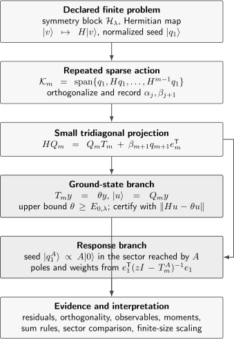
Lanczos is an evidence pipeline, not merely a recurrence. The ground-state branch is certified by Ritz residuals and observable convergence; the response branch is constrained by moments and sum rules. Both remain conditional on the declared sector and finite system.

Ritz Ground-State Approximation

Diagonalize the small matrix:

$$T_m y_i^{(m)} = \theta_i^{(m)}y_i^{(m)}, \qquad \|y_i^{(m)}\| = 1.$$

The corresponding Ritz vector in the many-body space is

$$|u_i^{(m)}\rangle = Q_m y_i^{(m)}.$$

Its Rayleigh quotient is exactly the Ritz value:

$$\frac{ \langle u_i^{(m)}|H|u_i^{(m)}\rangle }{ \langle u_i^{(m)}|u_i^{(m)}\rangle } = \theta_i^{(m)}.$$

For the lowest Ritz value, the variational principle gives

$$E_{0,\lambda} \le \theta_0^{(m)}.$$

Because exact-arithmetic Krylov spaces are nested,

$$\mathcal K_m \subseteq \mathcal K_{m+1},$$

the lowest Ritz values obey

$$E_{0,\lambda} \le \theta_0^{(m+1)} \le \theta_0^{(m)}.$$

Thus unrestarted exact-arithmetic Lanczos supplies a descending sequence of variational upper bounds within the chosen sector. Floating-point loss of orthogonality and restarted algorithms can obscure simple step-by-step monotonicity, so implementations should be judged by their documented convergence criteria rather than by this ideal property alone.

The residual is nearly free

Insert the projection identity into the Ritz equation:

$$\begin{aligned} |r_i^{(m)}\rangle &= H Q_m y_i^{(m)} - \theta_i^{(m)}Q_m y_i^{(m)} \\ &= \beta_{m+1} |q_{m+1}\rangle e_m^{\mathsf T}y_i^{(m)}. \end{aligned}$$

Therefore

$$\|r_i^{(m)}\| = \left| \beta_{m+1} e_m^{\mathsf T}y_i^{(m)} \right|.$$

No additional full Hamiltonian application is needed when the recurrence data are reliable. A direct recomputation of $H|u_i\rangle-\theta_i|u_i\rangle$ is nevertheless a valuable independent check for selected final states.

An absolute residual has units of energy. A useful scale-aware report includes, for example,

$$\rho_i = \frac{\|r_i\|}{ \max\left( \|H\|_{\mathrm{est}}, |\theta_i|, E_{\mathrm{scale}} \right)},$$

with the denominator stated explicitly. There is no universal tolerance divorced from the Hamiltonian scale and the accuracy required of downstream observables.

Energy variance is the same certificate

For a normalized Ritz vector, $\langle H\rangle=\theta_i$, so

$$\begin{aligned} \operatorname{Var}_{u_i}(H) &= \langle u_i| (H-\theta_i)^2 |u_i\rangle \\ &= \|r_i\|^2. \end{aligned}$$

Zero variance is equivalent to being an exact eigenvector of the represented Hermitian Hamiltonian. A small variance is a strong solver diagnostic, but it does not by itself identify which nearby eigenstate has been obtained when levels are clustered or degenerate.

Residuals and eigenvalue errors

For a normalized approximate eigenvector of a Hermitian matrix, at least one exact eigenvalue lies within the residual norm:

$$\min_n |E_{n,\lambda}-\theta_i| \le \|r_i\|.$$

This inclusion statement does not label the nearby eigenvalue. To bound a particular eigenvector or isolate a particular level, one also needs spectral separation and correct state identification. Near a degeneracy, a tiny residual can coexist with a rapidly rotating basis inside the nearly degenerate subspace.

What Controls Convergence

The full sector dimension $D_\lambda$ sets the worst-case ceiling, but it does not predict how many steps a useful calculation needs. Convergence depends on the spectral measure seen by the seed,

$$d\mu_{q_1}(E) = \sum_n |c_n|^2 \delta(E-E_{n,\lambda}),dE,$$

and therefore on several coupled features.

• Ground-state overlap: a very small $|c_0|$ delays the appearance of the ground-state component.
• Spectral separation: an isolated extremal level is generally easier to resolve than a dense low-energy cluster.
• Spectral width and distribution: polynomial separation depends on the placement of all eigenvalues carrying seed weight, not only on the first gap.
• Requested output: the energy may converge before long-range correlations, entanglement quantities, or small transition amplitudes.
• Finite precision: loss of orthogonality can generate duplicate Ritz values and spoil ideal recurrence identities.
• Restart policy: a bounded Krylov dimension controls memory but changes the convergence history and may discard useful directions.

It is therefore poor practice to prescribe a fixed number of Lanczos steps for every size and coupling. Stop when the relevant residuals and observables satisfy declared criteria, then show that tightening those criteria leaves the conclusions unchanged.

Energy convergence can be misleadingly early

Let a normalized trial state be

$$|\psi\rangle = \sqrt{1-\epsilon^2}|0\rangle + \epsilon|1\rangle,$$

with gap $\Delta=E_1-E_0>0$. Its energy error is

$$\langle H\rangle-E_0 = \epsilon^2\Delta,$$

whereas an observable with an off-diagonal matrix element can have a leading error proportional to $\epsilon$:

$$\begin{aligned} &\langle\psi|O|\psi\rangle - \langle0|O|0\rangle \\ &\qquad= 2\epsilon \operatorname{Re} \langle0|O|1\rangle \\ &\qquad\quad+ O(\epsilon^2). \end{aligned}$$

An apparently settled energy can therefore coexist with a less accurate observable. Production calculations should monitor the quantities used in the scientific claim, not only the Ritz value.

Worked Three-Level Example

Consider

$$H = \operatorname{diag}(0,1,2), \qquad |q_1\rangle = \frac{1}{\sqrt3} \begin{pmatrix} 1\\1\\1 \end{pmatrix}.$$

The first diagonal coefficient is

$$\alpha_1 = \langle q_1|H|q_1\rangle = 1.$$

After subtracting $\alpha_1|q_1\rangle$, normalization gives

$$\begin{gathered} \beta_2 = \sqrt{\frac23}, \\ |q_2\rangle = \frac{1}{\sqrt2} \begin{pmatrix} -1\\0\\1 \end{pmatrix}, \\ \alpha_2 = 1. \end{gathered}$$

Thus

$$T_2 = \begin{pmatrix} 1 & \sqrt{2/3} \\ \sqrt{2/3} & 1 \end{pmatrix},$$

with Ritz values

$$\theta_{\pm}^{(2)} = 1 \pm \sqrt{\frac23}.$$

The lower estimate is

$$\theta_-^{(2)} \approx 0.183503,$$

which is correctly above the exact ground energy $E_0=0$. The next recurrence coefficient is

$$\beta_3 = \frac{1}{\sqrt3}.$$

The normalized lower eigenvector of $T_2$ is $y_-=(1,-1)^{\mathsf T}/\sqrt2$, so the residual formula gives

$$\|r_-^{(2)}\| = \beta_3 \left| e_2^{\mathsf T}y_- \right| = \frac{1}{\sqrt6}.$$

The estimate is variational, but its residual is not yet small. At the third step,

$$T_3 = \begin{pmatrix} 1 & \sqrt{2/3} & 0 \\ \sqrt{2/3} & 1 & 1/\sqrt3 \\ 0 & 1/\sqrt3 & 1 \end{pmatrix},$$

whose eigenvalues are exactly $0$, $1$, and $2$. The Krylov space has reached the full spectral support of the seed, so the finite problem is recovered exactly.

This toy example illustrates three general points.

• A small projected matrix can already provide a useful upper bound.
• The residual quantifies how incomplete that estimate remains.
• Exact termination occurs after the number of distinct eigenvalues carrying seed weight, which can be much smaller than the ambient basis dimension in special cases.

Vectors, Memory, and Reconstruction

If only Ritz values and residual estimates are needed, the three-term recurrence can proceed while retaining only a few length-$D_\lambda$ vectors plus the scalar coefficients. A many-body observable usually requires a Ritz vector, however:

$$|u_i^{(m)}\rangle = \sum_{j=1}^{m} (y_i^{(m)})_j |q_j\rangle.$$

There are three common storage patterns.

Store the Krylov basis

Retaining all $m$ vectors permits direct Ritz-vector construction and full reorthogonalization. Its leading vector storage is

$$O(mD_\lambda).$$

This can dominate memory even when $T_m$ itself is tiny.

Reconstruct in a second pass

One can first save the recurrence coefficients, solve the small problem, then regenerate the Krylov sequence from the same seed and Hamiltonian action while accumulating the desired linear combination. This reduces stored-vector memory but approximately repeats the matrix-vector work. Exact reproducibility of the recurrence matters; nondeterministic parallel reductions and changed arithmetic order can complicate a naive second pass.

Restart or lock converged directions

Restarted methods cap the live subspace dimension, while locking preserves selected converged Ritz vectors. These strategies are essential in large calculations, but their details belong to Sparse Eigensolvers. A paper or notebook should identify the actual algorithm rather than using “Lanczos” as a catch-all label.

More Than One Low-Energy State

The extremal Ritz values of $T_m$ can approximate several low-lying eigenvalues at once. Their convergence is not uniform. The lowest state may settle while the next few states still exchange order or mix within a cluster.

For an exactly degenerate eigenspace $\mathcal D$, no numerical method is required to return a predetermined basis inside $\mathcal D$. The invariant object is the projector

$$P_{\mathcal D} = \sum_{a=1}^{g} |d_a\rangle\langle d_a|,$$

not any particular orthonormal set $\{|d_a\rangle\}$. Compare subspaces, symmetry labels, and projector-valued observables when individual vectors can rotate.

Several safeguards are useful when excited states matter.

• Request more Ritz pairs than the minimum needed near a suspected cluster.
• Resolve all commuting symmetries available before interpreting degeneracy.
• Check each residual, not only the ground-state residual.
• Compare stable invariant subspaces rather than raw eigenvector components.
• Use independent seeds or block methods when a single seed has poor support.
• Compare neighboring sectors before claiming a global gap or degeneracy.

Interior eigenstates are a harder target than spectral edges. A plain ground-state Lanczos run should not be presented as a generic finite-energy eigensolver.

Spectral Functions from a Second Lanczos Run

Once a normalized ground state $|0\rangle$ and energy $E_0$ are available, define the zero-temperature resolvent for an operator $A$:

$$\begin{aligned} G_A(z) &= \langle0| A^\dagger \bigl[z-(H-E_0)\bigr]^{-1} \\ &\qquad\times A|0\rangle, \\ \operatorname{Im}z &>0. \end{aligned}$$

The corresponding positive-frequency spectral measure is

$$\begin{aligned} S_A(\omega) &= \sum_n |\langle n|A|0\rangle|^2 \\ &\qquad\times \delta\!\left( \omega-E_n+E_0 \right). \end{aligned}$$

Its full physical interpretation and variants are developed in Spectral Functions. The comparative numerical workflow, including matched-kernel checks against direct sums and time evolution, is developed in Dynamical Correlation Functions Numerically. Lanczos enters through the response seed

$$|f_0\rangle = A|0\rangle, \qquad W_0 = \langle f_0|f_0\rangle.$$

If $W_0=0$, the spectrum vanishes for that state and operator. Otherwise choose

$$|q_1^{A}\rangle = \frac{|f_0\rangle}{\sqrt{W_0}}$$

and run Lanczos on $H-E_0$ in the sector reached by $A$. If the resulting tridiagonal coefficients are $a_j$ and $b_{j+1}$, the order-$m$ approximation is

$$\begin{gathered} G_A^{(m)}(z) = \cfrac{W_0}{ z-a_1 - \cfrac{b_2^2}{ z-a_2 -\ddots } }, \\ \text{terminal fraction:} \qquad \frac{b_m^2}{z-a_m}. \end{gathered}$$

Equivalently,

$$G_A^{(m)}(z) = W_0 e_1^{\mathsf T} (zI_m-T_m^A)^{-1} e_1.$$

If

$$T_m^A y_\ell = \vartheta_\ell y_\ell,$$

then

$$G_A^{(m)}(z) = W_0 \sum_{\ell=1}^{m} \frac{ |(y_\ell)_1|^2 }{z-\vartheta_\ell}.$$

The small tridiagonal problem therefore supplies both approximate pole locations and nonnegative weights.

The operator usually changes sector

If $|0\rangle$ lies in sector $\lambda_0$ and $A$ carries definite conserved quantum numbers, then

$$A: \mathcal H_{\lambda_0} \longrightarrow \mathcal H_{\lambda_A}.$$

For example, a momentum-$q$ operator maps a ground state of momentum $k_0$ to momentum $k_0+q$, while a particle-addition operator changes particle number by one. The ground-state run and the response run may therefore use different reduced bases. Applying the wrong sector representation can silently erase the signal or produce an invalid Hamiltonian action.

Broadening is a display and resolution choice

At finite size, the exact spectrum is a sum of delta functions. Evaluating at

$$z = \omega+i\eta, \qquad \eta>0,$$

gives a Lorentzian-broadened plot:

$$S_{A,\eta}^{(m)}(\omega) = -\frac{1}{\pi} \operatorname{Im} G_A^{(m)}(\omega+i\eta).$$

For discrete poles this is

$$\begin{aligned} S_{A,\eta}^{(m)}(\omega) &= W_0 \sum_\ell |(y_\ell)_1|^2 \\ &\qquad\times \frac{1}{\pi} \frac{\eta}{ (\omega-\vartheta_\ell)^2+\eta^2 }. \end{aligned}$$

Unless a physical self-energy or coupling to an environment has been included, $\eta$ is not a measured lifetime. It is a numerical resolution parameter. A reproducible spectrum reports $\eta$, the line shape, system size, boundary conditions, sector, frequency grid, and whether the displayed features persist when these choices are varied.

Moments and sum rules

The zeroth moment is exact by construction:

$$\int_{-\infty}^{\infty} S_A(\omega),d\omega = W_0 = \langle0|A^\dagger A|0\rangle.$$

More generally, define

$$\mu_p = \langle f_0| (H-E_0)^p |f_0\rangle.$$

In exact arithmetic, the $m$-step Lanczos quadrature obeys

$$\mu_p = W_0 e_1^{\mathsf T} (T_m^A)^p e_1, \qquad 0\le p\le 2m-1,$$

provided the Krylov process has not terminated earlier. This moment-matching property explains why a modest tridiagonal representation can reproduce integrated spectral information before every individual finite-size pole has converged.

Use independent operator identities from Sum Rules as validation tests. A visually smooth curve is much weaker evidence than correct nonnegative weights, moments, and integrated spectral weight.

Finite-Precision Failure Modes

The elegant three-term recurrence assumes exact arithmetic. Real calculations require an explicit policy for roundoff.

Loss of orthogonality and ghost Ritz values

As extremal Ritz pairs converge, floating-point Lanczos vectors tend to lose mutual orthogonality. The projected calculation can then rediscover an already converged direction and produce repeated or “ghost” Ritz values. A duplicate number in $T_m$ is not evidence for a physical degeneracy.

Possible responses include full reorthogonalization, selective or partial reorthogonalization, locking converged vectors, and carefully designed restarted methods. Each trades memory, orthogonalization cost, and robustness. Relevant diagnostics include

$$\|Q_m^\dagger Q_m-I_m\|,$$

independently recomputed residuals, and stability under a stricter orthogonality policy.

Small overlap and false absence

If the desired state has exactly zero seed overlap, it is mathematically inaccessible. If the overlap is merely tiny, the state may appear only after many iterations and can be lost amid roundoff or restart filtering. Multiple independent seeds and symmetry-aware seeds help distinguish genuine spectral absence from poor sampling of the invariant subspace.

Near-degenerate clusters

Individual Ritz vectors can rotate strongly while the low-energy invariant subspace is already accurate. Compare projectors, principal angles, or symmetry-resolved matrix elements rather than demanding componentwise agreement between arbitrary bases of the same cluster.

Interior states and dense spectra

Plain Lanczos favors spectral edges. High-energy or interior states in a many-body spectrum can be surrounded by exponentially many nearby levels. Shift-invert or polynomial filtering may improve targeting, but factorization cost, conditioning, and memory can become decisive. These are different computational regimes, not minor settings on a ground-state run.

Nondeterministic arithmetic

Parallel sparse matrix-vector products and reductions may change summation order between runs. Bitwise-identical Ritz vectors are then an inappropriate reproducibility criterion, especially inside degenerate subspaces. Residuals, invariant quantities, and stated numerical tolerances are the meaningful comparison targets.

Non-Hermitian operators

The standard real-symmetric or Hermitian Lanczos structure does not apply unchanged to a generic non-Hermitian matrix. Arnoldi, biorthogonal Lanczos variants, or specialized structure-preserving methods are needed, with different stability questions. Do not use a Hermitian residual or variational interpretation outside its assumptions.

Physical Limitations After Numerical Convergence

A converged Krylov calculation can still answer the wrong physical question.

One sector is not the global spectrum

Lanczos finds the lowest state visible in the chosen invariant block. The global finite-system ground state is

$$E_0 = \min_\lambda E_{0,\lambda}.$$

If the winning sector is not known analytically, compare all plausible sectors. Crossings between sector minima can be physical and should not be hidden by fixing labels too early.

One size is not a phase

An essentially exact ground state on one cluster does not establish long-range order, a thermodynamic gap, or a phase transition. Those claims require controlled size sequences, compatible geometries, and a dedicated finite-size-scaling analysis.

A few states are not a thermal trace

Low-temperature observables may be dominated by a small spectral window, but a complete finite-temperature trace is

$$\langle O\rangle_\beta = \frac{ \sum_n e^{-\beta E_n} \langle n|O|n\rangle }{ \sum_n e^{-\beta E_n} }.$$

A handful of low Ritz pairs is not generally enough at moderate or high temperature. Finite-temperature Lanczos methods add stochastic trace estimation and further approximations; they must be documented separately.

A broadened finite spectrum is not automatically a continuum

The apparent smoothness of $S_{A,\eta}(\omega)$ depends on $\eta$, level spacing, geometry, and system size. Features narrower than the finite-size spacing or comparable to the chosen broadening need a scaling study before receiving a continuum interpretation.

Validation Ladder

A defensible Lanczos calculation can be audited in layers.

1. Basis and sector checks

• Reproduce the declared sector dimension independently.
• Verify that $H|v\rangle$ never leaves the sector.
• Confirm Hermiticity through matrix elements or randomized bilinear tests.
• Check simple traces or moments on small sectors where they are available.

2. Solver checks

• Report absolute and scaled residuals for every used Ritz pair.
• Tighten the iteration and orthogonality settings.
• Recompute selected residuals directly in the full sector representation.
• Compare independent start vectors when overlap is uncertain.
• Monitor duplicate Ritz values and basis orthogonality when applicable.

3. Observable checks

• Increase the Krylov dimension or tighten restart tolerances until claimed observables stabilize.
• Verify exact symmetries and selection rules.
• Check normalization, positivity, moments, and spectral sum rules.
• Compare equivalent operator formulations when available.

4. Small-system benchmarks

On a sector small enough for complete diagonalization, compare

$$\begin{gathered} \text{energies and residuals}, \\ \text{eigenstate observables}, \\ \text{transition weights}, \\ \text{spectral moments}. \end{gathered}$$

This tests basis conventions, fermionic signs, sector maps, and observable kernels together with the eigensolver.

5. Physical scaling checks

• Compare system sizes and compatible cluster shapes.
• Vary boundary conditions or twists when physically appropriate.
• Separate solver uncertainty from finite-size drift.
• State which conclusions are finite-system facts and which are extrapolations.

Validation Tests provides the broader reference checklist for numerical claims.

Reproducibility Record

A useful Lanczos result should preserve enough information to rerun both the finite problem and the solver.

• Hamiltonian formula, parameter values, units, and energy offset.
• Geometry, site ordering, boundary conditions, and local cutoff.
• Basis convention and every enforced symmetry label.
• Sector dimension and Hamiltonian storage or matrix-free action.
• Solver implementation and version.
• Start-vector construction and random seed.
• Requested Ritz pairs, Krylov dimension, restart and locking policy.
• Reorthogonalization policy and floating-point precision.
• Stopping criteria, iteration count, and final residuals.
• Observable convergence data and independent checks.
• For spectra: operator convention, target sector, frequency grid, broadening kernel, $\eta$, moments, and sum-rule errors.
• Hardware and parallel settings when nondeterministic reductions or performance claims matter.

The record should distinguish a solver tolerance from the actual achieved residual and both from the estimated physical uncertainty.

Common Mistakes

Calling a Ritz value exact because many digits stopped changing

Digit stability is not an eigenpair test. Report the residual and show convergence of the observables used.

Forgetting the sector qualifier

The lowest state in a fixed particle-number or momentum block need not be the global ground state. Compare sectors or justify the restriction analytically.

Treating repeated Ritz values as degeneracy

Loss of orthogonality can create ghost copies. Check symmetry labels, independent residuals, invariant subspaces, and the orthogonalization policy.

Using the wrong response sector

The seed $A|0\rangle$ carries the quantum numbers of $A$. Build the target basis accordingly.

Interpreting the broadening as a lifetime

A plotting parameter $\eta$ is not a decay rate unless the physical model supplies that interpretation.

Checking only the ground-state energy

Correlators and transition amplitudes can converge more slowly than the energy. Monitor the quantities that support the conclusion.

Expecting plain Lanczos to resolve the whole spectrum

The method is especially effective for a few spectral-edge states and seed-weighted response information. It does not remove the exponential size of a generic many-body spectrum.

Hiding algorithmic choices behind the word Lanczos

Unrestarted, restarted, thick-restart, block, and differently reorthogonalized implementations have different memory and reliability profiles. Name the method actually used.

Exercises

1. Shift invariance and missing support

Prove that

$$\mathcal K_m(H-\sigma I,q) = \mathcal K_m(H,q).$$

Then show that if $\langle n|q\rangle=0$ for an eigenvector $|n\rangle$ of $H$, every vector in either Krylov space is orthogonal to $|n\rangle$.

Solution

The binomial theorem gives

$$(H-\sigma I)^j q = \sum_{k=0}^{j} \binom{j}{k} (-\sigma)^{j-k} H^kq.$$

Thus each generator of $\mathcal K_m(H-\sigma I,q)$ belongs to $\mathcal K_m(H,q)$. Replacing $H$ by $(H-\sigma I)+\sigma I$ gives the reverse inclusion, so the spaces are equal.

If

$$H|n\rangle = E_n|n\rangle, \qquad \langle n|q\rangle = 0,$$

then

$$\langle n|H^k|q\rangle = E_n^k \langle n|q\rangle = 0$$

for every nonnegative integer $k$. Every linear combination of the Krylov generators is therefore orthogonal to $|n\rangle$. A scalar shift cannot repair missing seed support.

2. Two Lanczos steps for three levels

For

$$H = \operatorname{diag}(0,1,2), \qquad q_1 = \frac{1}{\sqrt3}(1,1,1)^{\mathsf T},$$

derive $\alpha_1$, $\beta_2$, $q_2$, $\alpha_2$, and the two Ritz values. Explain why the lower Ritz value cannot lie below zero.

Solution

First,

$$\alpha_1 = q_1^\dagger Hq_1 = 1.$$

The unnormalized next vector is

$$w_1 = Hq_1-\alpha_1q_1 = \frac{1}{\sqrt3} (-1,0,1)^{\mathsf T}.$$

Hence

$$\begin{gathered} \beta_2 = \|w_1\| = \sqrt{\frac23}, \\ q_2 = \frac{1}{\sqrt2} (-1,0,1)^{\mathsf T}. \end{gathered}$$

The second diagonal coefficient is

$$\alpha_2 = q_2^\dagger Hq_2 = 1.$$

Therefore

$$T_2 = \begin{pmatrix} 1 & \sqrt{2/3} \\ \sqrt{2/3} & 1 \end{pmatrix},$$

and

$$\theta_\pm = 1\pm\sqrt{\frac23}.$$

The lower value is about $0.183503$. It is the minimum Rayleigh quotient over the two-dimensional Krylov subspace. Since the exact minimum over the full space is $E_0=0$, restricting the minimization cannot produce a smaller value.

3. Residual and variance identity

Starting from

$$HQ_m = Q_mT_m + \beta_{m+1}q_{m+1}e_m^{\mathsf T},$$

derive the Ritz residual formula. Then prove that the energy variance of a normalized Ritz vector equals the squared residual norm.

Solution

Let

$$T_my = \theta y, \qquad u = Q_my.$$

Then

$$\begin{aligned} Hu-\theta u &= HQ_my-Q_mT_my \\ &= \beta_{m+1} q_{m+1} e_m^{\mathsf T}y. \end{aligned}$$

Because $q_{m+1}$ is normalized,

$$\|Hu-\theta u\| = \left| \beta_{m+1}e_m^{\mathsf T}y \right|.$$

Also,

$$\langle u|H|u\rangle = y^\dagger T_my = \theta.$$

For normalized $u$ and Hermitian $H$,

$$\begin{aligned} \operatorname{Var}_u(H) &= \langle u|(H-\theta)^2|u\rangle \\ &= \langle (H-\theta)u|(H-\theta)u\rangle \\ &= \|Hu-\theta u\|^2. \end{aligned}$$

4. Zeroth spectral sum rule

Let

$$\begin{aligned} S_A(\omega) &= \sum_n |\langle n|A|0\rangle|^2 \\ &\qquad\times \delta(\omega-E_n+E_0). \end{aligned}$$

Show that its total weight is $\langle0|A^\dagger A|0\rangle$. Then show that the $m$-pole Lanczos representation has the same total weight.

Solution

Integrating and inserting completeness gives

$$\begin{aligned} \int d\omega\,S_A(\omega) &= \sum_n \langle0|A^\dagger|n\rangle \\ &\qquad\times \langle n|A|0\rangle \\ &= \langle0|A^\dagger \left( \sum_n|n\rangle\langle n| \right) \\ &\qquad\times A|0\rangle \\ &= \langle0|A^\dagger A|0\rangle \\ &= W_0. \end{aligned}$$

The Lanczos pole weights are

$$w_\ell = W_0|(y_\ell)_1|^2.$$

Because the eigenvectors of $T_m^A$ form an orthonormal basis,

$$\sum_\ell |(y_\ell)_1|^2 = e_1^{\mathsf T}I_me_1 = 1.$$

Therefore

$$\sum_\ell w_\ell = W_0.$$

This check can pass even when individual poles have not converged, so it complements rather than replaces frequency-resolved tests.

5. Diagnose a claimed degeneracy

A computation in one symmetry block reports three nearly identical lowest Ritz values, but the associated Lanczos vectors have lost orthogonality. Design a minimal sequence of checks that distinguishes a physical threefold degeneracy from ghost Ritz values.

Solution

A defensible sequence is:

1. Reconstruct all three Ritz vectors and directly recompute their residuals.
2. Measure their mutual overlaps and, if the Krylov basis was stored, $\|Q_m^\dagger Q_m-I\|$.
3. Repeat with full or stricter selective reorthogonalization and locking of converged directions.
4. Use independent start vectors or a block method so the candidate subspace is sampled in more than one way.
5. Resolve every available commuting symmetry and check whether the states carry distinct labels.
6. Compare the projector onto the candidate three-dimensional subspace across solver settings.
7. Benchmark a smaller related sector against complete diagonalization.

If the multiplicity disappears under reorthogonalization or the putative vectors collapse onto the same direction, the repeated values were numerical ghosts. If three linearly independent, small-residual states persist and their invariant subspace is stable, the evidence supports a physical degeneracy of the represented finite problem. Establishing a thermodynamic degeneracy still requires finite-size analysis.

References

• C. Lanczos, “An Iteration Method for the Solution of the Eigenvalue Problem of Linear Differential and Integral Operators,” Journal of Research of the National Bureau of Standards 45, 255–282 (1950), doi:10.6028/jres.045.026.
• C. C. Paige, “Error Analysis of the Lanczos Algorithm for Tridiagonalizing a Symmetric Matrix,” Journal of the Institute of Mathematics and Its Applications 18, 341–349 (1976), doi:10.1093/imamat/18.3.341.
• B. N. Parlett and D. S. Scott, “The Lanczos Algorithm with Selective Orthogonalization,” Mathematics of Computation 33, 217–238 (1979), doi:10.1090/S0025-5718-1979-0514820-3.
• J. K. Cullum and R. A. Willoughby, Lanczos Algorithms for Large Symmetric Eigenvalue Computations, Birkhäuser, 1985.
• Y. Saad, Numerical Methods for Large Eigenvalue Problems, revised edition, SIAM, 2011, doi:10.1137/1.9781611970739.
• H. Q. Lin, “Exact Diagonalization of Quantum-Spin Models,” Physical Review B 42, 6561–6567 (1990), doi:10.1103/PhysRevB.42.6561.
• E. Dagotto, “Correlated Electrons in High-Temperature Superconductors,” Reviews of Modern Physics 66, 763–840 (1994), doi:10.1103/RevModPhys.66.763.
• E. R. Gagliano and C. A. Balseiro, “Dynamical Properties of Quantum Many-Body Systems at Zero Temperature,” Physical Review Letters 59, 2999–3002 (1987), doi:10.1103/PhysRevLett.59.2999.
• E. R. Gagliano and C. A. Balseiro, “Dynamic Correlation Functions in Quantum Many-Body Systems at Zero Temperature,” Physical Review B 38, 11766–11773 (1988), doi:10.1103/PhysRevB.38.11766.
• R. Haydock, V. Heine, and M. J. Kelly, “Electronic Structure Based on the Local Atomic Environment for Tight-Binding Bands,” Journal of Physics C: Solid State Physics 5, 2845–2858 (1972), doi:10.1088/0022-3719/5/20/004.
• J. Jaklič and P. Prelovšek, “Finite-Temperature Properties of Doped Antiferromagnets,” Advances in Physics 49, 1–92 (2000), doi:10.1080/000187300243381.
• A. W. Sandvik, “Computational Studies of Quantum Spin Systems,” in AIP Conference Proceedings 1297, 135–338 (2010), doi:10.1063/1.3518900.

Further Study

• Computational Many-Body Overview
• Dynamical Correlation Functions Numerically
• Exact Diagonalization Preview
• Symmetry Sectors in Many-Body Numerics
• Scaling of Hilbert Space
• Sparse Matrices
• Sparse Eigensolvers
• Upper Bounds and the Min–Max Principle
• Spectral Functions
• Sum Rules
• Validation Tests