Quantum Monte Carlo Preview

Quantum Monte Carlo replaces an exponentially large quantum sum by stochastic sampling of a carefully chosen configuration representation. When the configuration weights are nonnegative and updates explore them efficiently, equilibrium observables of systems far larger than exact diagonalization can be estimated without a mean-field or small-coupling approximation. The result is nevertheless not “exact because it is Monte Carlo”: it carries statistical uncertainty, autocorrelation, equilibration risk, finite-size and finite-temperature effects, and any discretization or representation errors introduced before sampling.

For a thermal target,

$$\begin{aligned} Z(\beta) &= \operatorname{Tr}e^{-\beta H}, \\ \langle O\rangle_\beta &= \frac{ \operatorname{Tr} \left( Oe^{-\beta H} \right) }{ Z(\beta) }. \end{aligned}$$

The central QMC move is to rewrite these quantities as a sum or integral over configurations $C$,

$$\begin{aligned} Z &= \sum_C W(C), \\ \langle O\rangle &= \frac{ \sum_C W(C)O_{\mathrm{est}}(C) }{ \sum_C W(C) }. \end{aligned}$$

If $W(C)\ge 0$, the normalized weight can be treated as a probability and sampled by a Markov chain. If the weights fluctuate in sign or phase, the same algebra remains true but the statistical problem can become exponentially hard.

Purpose and canonical scope

This page owns the many-body computational preview of equilibrium quantum Monte Carlo:

• how thermal traces become time-sliced paths, worldlines, operator strings, or auxiliary fields;
• what a sampled configuration means physically and what it does not mean;
• how importance sampling and nonlocal updates produce correlated data;
• how observables are represented by estimators;
• how statistical and systematic uncertainties are separated;
• how a QMC result is validated and reported.

Generic probability, importance sampling, sample means, and Markov-chain concepts have their canonical home in Monte Carlo Basics. The derivation and boundary conditions of the many-body functional integral belong to Path Integrals for Many-Body Systems. Finite-Size Scaling in Numerics owns thermodynamic extrapolation, and Analytic Continuation owns real-frequency inference from Euclidean data.

The Sign Problem Preview treats cancellation, basis dependence, sign-free structures, and exponential sampling cost in depth. Here the obstruction appears only far enough to mark the boundary of probability sampling.

Quantum Monte Carlo is a family

The name QMC covers methods with different sampled objects and different biases.

Path-integral Monte Carlo samples coordinate paths or ring-polymer configurations, often for continuum particles. Exchange appears through permutations of worldline endpoints.

Worldline and loop methods sample local-basis histories of spins, bosons, or other lattice degrees of freedom. Kinks represent off-diagonal operator events.

Stochastic series expansion samples terms in the power-series expansion of $e^{-\beta H}$, usually as an operator string acting on a basis state. It has no imaginary-time step.

Auxiliary-field or determinant QMC decouples interactions with Hubbard–Stratonovich fields, integrates quadratic fermions, and samples a determinant-dependent field configuration.

Projector, diffusion, and reptation methods extract ground-state information by imaginary-time projection. Trial-state constraints can introduce distinct biases.

Variational Monte Carlo samples a chosen trial wavefunction rather than a partition-function representation. Its canonical preview is Variational Monte Carlo.

This article centers finite-temperature partition-function methods because they make the common logic especially transparent. An algorithm must still state its representation, ensemble, update family, estimator, and controlled limits; “QMC” alone is not a reproducible method description.

The representation-to-evidence chain

A useful calculation keeps six layers distinct:

1. Physical target: $H$, $\beta$, geometry, boundary conditions, ensemble, and observable.
2. Exact identity: trace, series, path integral, or auxiliary-field transformation.
3. Controlled approximation: time step, basis cutoff, projection length, or stabilization scheme.
4. Sampling process: configuration space, proposal moves, stationary weight, and ergodic sectors.
5. Estimator and uncertainty: autocorrelation-aware mean, covariance, and nonlinear error propagation.
6. Physical limits: time-step, projection, size, temperature, and continuation analysis.

The reported number is trustworthy only when all six layers are auditable.

Suppose the desired thermodynamic value is $O_\infty$. A compact error decomposition is

$$\begin{aligned} \widehat O &= O_\infty +\delta_{\mathrm{MC}} +\delta_{\mathrm{eq}} \\ &\quad +\delta_{\Delta\tau} +\delta_{\beta} \\ &\quad +\delta_L +\delta_{\mathrm{other}}. \end{aligned}$$

Only $\delta_{\mathrm{MC}}$ is ordinary finite-sample fluctuation. More samples do not automatically remove the other terms.

From a trace to worldlines

For distinguishable continuum particles with collective coordinate $R$, the thermal density matrix is

$$\rho(R,R';\beta) = \langle R| e^{-\beta H} |R'\rangle.$$

Splitting $\beta=M\Delta\tau$ and inserting intermediate coordinates produces

$$\begin{aligned} \rho(R_0,R_M;\beta) &= \int dR_1\cdots dR_{M-1} \\ &\quad\times \prod_{\ell=0}^{M-1} \rho(R_\ell,R_{\ell+1};\Delta\tau). \end{aligned}$$

Each sequence $(R_0,\ldots,R_M)$ is a discretized imaginary-time path. Taking the trace identifies $R_M=R_0$. For identical particles, the trace closes up to a permutation $P$:

$$\begin{aligned} Z_N^{(\pm)} &= \frac{1}{N!} \sum_P (\pm1)^P \\ &\quad\times \int dR\, \rho(R,PR;\beta). \end{aligned}$$

The plus sign describes bosonic exchange; the permutation parity produces fermionic signs in a coordinate representation.

On a lattice, insert occupation-number or spin basis states instead of coordinates. A configuration then records a basis label on each imaginary-time slice. Diagonal evolution preserves the label, while an off-diagonal operator creates a kink or hop.

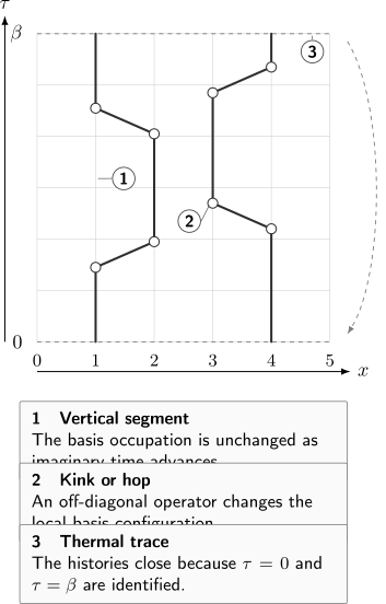
A local-basis worldline configuration. Vertical segments preserve occupation as imaginary time advances; diagonal segments mark hopping events. The thermal trace identifies $\tau=0$ and $\tau=\beta$. These paths are terms in a Euclidean representation, not literal real-time trajectories.

What the extra dimension means

A $d$-dimensional quantum system can resemble a $(d+1)$-dimensional anisotropic classical system, with compact imaginary time as the additional direction. This correspondence is structural, but several cautions matter:

• imaginary time has circumference $\beta$, not an independently infinite spatial extent;
• temporal and spatial couplings are generally anisotropic;
• bosonic and fermionic fields have different thermal boundary conditions;
• worldline permutations encode exchange;
• the Markov-chain step used to update a configuration is not the coordinate $\tau$;
• neither imaginary time nor Monte Carlo time is physical real time.

The complete boundary-condition ledger is developed in Path Integrals for Many-Body Systems.

Worked mapping: transverse-field Ising model

Consider

$$H = -J \sum_{\langle ij\rangle} \sigma_i^z\sigma_j^z -\Gamma \sum_i \sigma_i^x.$$

Write $H=H_z+H_x$, where $H_z$ is diagonal in the $\sigma^z$ basis. With $\Delta\tau=\beta/M$, a symmetric product formula gives

$$\begin{aligned} e^{-\Delta\tau(H_z+H_x)} &= e^{-\Delta\tau H_z/2} e^{-\Delta\tau H_x} e^{-\Delta\tau H_z/2} \\ &\quad +O(\Delta\tau^3). \end{aligned}$$

After $M$ factors, smooth thermodynamic quantities generally have a leading global error of order $\Delta\tau^2$ for this symmetric decomposition.

Let

$$\sigma_i^z |\{s\}_\ell\rangle = s_{i,\ell} |\{s\}_\ell\rangle, \qquad s_{i,\ell}=\pm1.$$

The spatial part contributes

$$\exp\!\left[ K_s \sum_{\langle ij\rangle} s_{i,\ell}s_{j,\ell} \right], \qquad K_s=J\Delta\tau.$$

At one site, put $a=\Gamma\Delta\tau$. The temporal transfer matrix is

$$\langle s'| e^{a\sigma^x} |s\rangle = \begin{cases} \cosh a, & s'=s,\\ \sinh a, & s'=-s. \end{cases}$$

It can be written as

$$\langle s'| e^{a\sigma^x} |s\rangle = C e^{K_\tau ss'},$$

where

$$\begin{aligned} K_\tau &= \frac{1}{2} \ln\coth a, \\ C &= \left( \frac{1}{2}\sinh 2a \right)^{1/2}. \end{aligned}$$

The time-sliced partition function is therefore

$$\begin{aligned} Z_M &= C^{NM} \sum_{\{s_{i,\ell}\}} \exp \Biggl[ K_s \sum_{\ell,\langle ij\rangle} s_{i,\ell}s_{j,\ell} \\ &\qquad\qquad +K_\tau \sum_{\ell,i} s_{i,\ell}s_{i,\ell+1} \Biggr], \end{aligned}$$

with

$$s_{i,M} = s_{i,0}.$$

Thus the quantum model maps to an anisotropic classical Ising model with periodic imaginary time. As $\Delta\tau\to0$, $K_s\to0$ while $K_\tau\to\infty$; neighboring time slices become strongly correlated. This makes naive single-spin updates inefficient and motivates continuous-time, cluster, or loop formulations.

What is exact in the mapping?

For finite $M$, the insertion of basis states and evaluation of each transfer-matrix element are exact. The symmetric product formula is approximate. Monte Carlo sampling adds statistical error. The physical thermodynamic limit adds finite-$L$ analysis.

The limits should be written separately:

$$\langle O\rangle = \lim_{L\to\infty} \lim_{\Delta\tau\to0} \widehat O_{L,\Delta\tau,\beta},$$

with a further $\beta\to\infty$ limit only when a ground-state observable is desired. Whether these limits commute must be checked rather than presumed.

Stochastic series expansion

Time slicing is not the only route. Expand

$$e^{-\beta H} = \sum_{n=0}^{\infty} \frac{(-\beta H)^n}{n!}.$$

Suppose

$$H = - \sum_b H_b$$

in a basis where the relevant products have nonnegative matrix elements. Inserting basis states gives

$$\begin{aligned} Z &= \sum_\alpha \sum_{n=0}^{\infty} \frac{\beta^n}{n!} \sum_{b_1,\ldots,b_n} \\ &\quad\times \left\langle\alpha\right| H_{b_1}\cdots H_{b_n} \left|\alpha\right\rangle. \end{aligned}$$

A configuration consists of the state $|\alpha\rangle$, the expansion order $n$, and an ordered operator sequence. Implementations often pad the sequence with identity operators to a variable or fixed maximum length. Operator-loop or directed-loop updates alter extended portions of the sequence and propagated basis states.

SSE has no Trotter step. It can still have:

• truncation risk if the allocated operator-string length is too short;
• autocorrelation and equilibration error;
• a sign problem if matrix elements do not define nonnegative weights;
• finite-$L$ and finite-$\beta$ effects;
• estimator and implementation errors.

Expansion-order estimators

Because every order-$n$ term carries $\beta^n$,

$$E = -\frac{\partial\ln Z}{\partial\beta} = -\frac{\langle n\rangle}{\beta},$$

when no constant Hamiltonian shift has been hidden in the decomposition. If $H$ was shifted, restore that known constant.

In units with $k_{\mathrm B}=1$, the heat capacity is

$$C_V = \langle n^2\rangle -\langle n\rangle^2 -\langle n\rangle.$$

These identities illustrate an important QMC principle: a good representation can turn a difficult operator expectation into a low-variance statistic of the sampled configuration.

Auxiliary-field and determinant sampling

For interacting fermions, one can split imaginary time, decouple a quartic interaction with an auxiliary field, and integrate the now-quadratic fermions. Schematically,

$$Z = \sum_{\{s\}} W_{\mathrm B}[s]\, \det M_\uparrow[s]\, \det M_\downarrow[s].$$

The sampled object is the auxiliary field $s$, not a set of classical fermion trajectories. Matrix products over many time slices can become badly conditioned, so QR, singular-value, or related stabilization is part of the numerical definition.

In special symmetry settings, the determinant product is nonnegative. In others, it fluctuates in sign or phase. The Hubbard–Stratonovich Transformation owns the decoupling identities, channel choices, determinant structure, and contour cautions.

Importance sampling

Assume $W(C)\ge0$ and define

$$\pi(C) = \frac{W(C)}{Z}.$$

Direct independent sampling from $\pi$ is usually unavailable. A Markov chain uses a transition kernel $P(C\to C')$ whose stationary distribution is $\pi$.

Detailed balance,

$$\pi(C)P(C\to C') = \pi(C')P(C'\to C),$$

is a sufficient condition for stationarity, though not a logically necessary one.

If $q(C\to C')$ proposes a move, the Metropolis–Hastings acceptance probability is

$$\begin{aligned} A(C\to C') &= \min \Biggl[ 1, \\ &\quad \frac{ W(C')q(C'\to C) }{ W(C)q(C\to C') } \Biggr]. \end{aligned}$$

For a symmetric proposal, only the weight ratio remains. Computing that ratio locally and stably is often the core implementation task.

Stationarity is not enough

An invariant distribution is useful only if the chain reaches and explores it. The update set must be irreducible over every sector intended to contribute. Slow mixing can arise from:

• critical fluctuations;
• large free-energy barriers;
• winding or topological sectors;
• conserved particle number;
• nearly frozen imaginary-time strands;
• determinant fields with widely separated scales;
• first-order phase coexistence.

A chain trapped in one sector may produce smooth time series and tiny within-sector error bars while estimating the wrong ensemble.

Update families

Local updates

A local move changes one field, spin, vertex, kink, or short path segment. It is simple to validate because the acceptance ratio depends on a local weight ratio. But local moves can decorrelate long-wavelength modes extremely slowly.

Cluster and loop updates

Cluster or loop algorithms build an extended object using local probabilities and flip it collectively. They can reduce critical slowing down dramatically when the representation admits a useful graph decomposition. Their efficiency is model- and parameter-dependent; a large cluster is not automatically an independent sample.

Worm updates

A worm algorithm temporarily enlarges configuration space to include two discontinuities. Moving one endpoint updates a worldline or graph while directly sampling a two-point function. When the endpoints meet, the configuration returns to the partition-function sector.

The enlarged ensemble needs a declared relative normalization. Measurements in the open and closed sectors answer different estimator questions.

Global field moves

Auxiliary-field methods may use delayed updates, force-biased proposals, global molecular-dynamics trajectories, or other collective moves. Acceptance and reversibility tests must include every approximation used to compute determinant ratios or forces.

Estimators

An estimator is a function of the sampled configuration whose ensemble expectation equals the target observable. It is part of the algorithm, not an afterthought.

Diagonal observables

For a worldline basis in which $O$ is diagonal, one may average $O$ over imaginary-time slices:

$$O_{\mathrm{est}}(C) = \frac{1}{M} \sum_{\ell=0}^{M-1} O(\alpha_\ell).$$

Time-translation symmetry improves statistics, but measurements at different slices of the same configuration are correlated.

Derivative estimators

If a parameter $\lambda$ appears in $H$, then

$$\frac{\partial\ln Z}{\partial\lambda} = - \int_0^\beta d\tau\, \left\langle \frac{\partial H(\tau)}{\partial\lambda} \right\rangle.$$

In a series or graph representation, this derivative can become a count of selected operators or vertices. Susceptibilities similarly become fluctuations or integrated correlations.

Off-diagonal observables

Off-diagonal correlations generally require operator insertions, open-worldline sectors, Green-function estimators, or improved loop estimators. Simply reading a diagonal basis label does not estimate a noncommuting operator.

Winding estimators

With periodic spatial boundaries, worldline winding fluctuations can diagnose superfluid stiffness. The proportionality factor among $\rho_s$, $\langle\mathbf W^2\rangle$, $\beta$, mass, dimension, and system lengths depends on units and geometry. State the convention rather than quoting only a winding number.

Superfluidity in Condensed Matter applies a convention-declared winding estimator to physical neutral-superfluid claims; this page retains estimator, autocorrelation, and finite-size validity checks.

Euclidean correlators

QMC naturally produces equal-time or imaginary-time quantities such as

$$G(\tau) = \left\langle T_\tau A(\tau)B(0) \right\rangle_\beta.$$

This is not a real-time correlator. Recovering a spectral function generally requires an ill-conditioned inverse problem; a small error bar on $G(\tau)$ does not imply a uniquely resolved real-frequency peak.

Statistical errors from correlated samples

After equilibration, let

$$Y_t = O_{\mathrm{est}}(C_t), \qquad \overline Y = \frac{1}{N_{\mathrm{meas}}} \sum_{t=1}^{N_{\mathrm{meas}}}Y_t.$$

Define the stationary autocovariance and normalized autocorrelation by

$$\begin{aligned} \Gamma_Y(k) &= \left\langle (Y_t-\mu_Y) (Y_{t+k}-\mu_Y) \right\rangle, \\ \rho_Y(k) &= \frac{\Gamma_Y(k)}{\Gamma_Y(0)}. \end{aligned}$$

With the convention

$$\tau_{\mathrm{int},Y} = \frac{1}{2} +\sum_{k=1}^{\infty}\rho_Y(k),$$

the asymptotic variance of the mean is

$$\operatorname{Var}(\overline Y) \approx \frac{ 2\tau_{\mathrm{int},Y}\Gamma_Y(0) }{ N_{\mathrm{meas}} }.$$

An effective independent sample count is therefore

$$N_{\mathrm{eff},Y} \approx \frac{ N_{\mathrm{meas}} }{ 2\tau_{\mathrm{int},Y} }.$$

Autocorrelation time is observable-dependent. Energy can decorrelate rapidly while a winding number or order parameter remains nearly frozen.

Estimating autocorrelation

At large lag, the empirical autocorrelation is mostly noise. Summing it to the end of a run is unstable; truncating too early misses slow modes. Practical analyses use a self-consistent window, blocking or batch means, and independent chains. Report the rule used.

Thinning a chain discards data and is not a substitute for estimating $\tau_{\mathrm{int}}$. It may reduce storage, but a correctly analyzed unthinned chain usually contains at least as much information.

Nonlinear derived quantities

Ratios, Binder cumulants, fitted gaps, reweighted estimates, and crossing locations are nonlinear functions of correlated primary measurements. Propagate their joint covariance by blocked bootstrap, jackknife, or a justified delta method. Resampling individual measurements without preserving blocks destroys the time correlation.

Equilibration

Discarding a fixed number of initial sweeps does not prove equilibrium. Useful evidence includes:

• chains started from ordered, disordered, and sector-distinct configurations;
• agreement of late-time means among independent seeds;
• stabilization of histograms and slow observables;
• round trips between relevant sectors or phases;
• run lengths many times larger than the largest measured autocorrelation time;
• consistency between forward and reverse parameter scans;
• replica-exchange or tempering diagnostics when those methods are used.

An acceptance rate near one can indicate tiny proposals that mix poorly. An acceptance rate near zero indicates mostly rejected proposals. Neither rate alone measures effective sample size.

Systematic limits

Imaginary-time discretization

If a symmetric factorization has leading error

$$O(\Delta\tau) = O_0+c_2\Delta\tau^2+\cdots,$$

simulate several time steps and extrapolate against $\Delta\tau^2$. The coefficient and asymptotic window are observable-dependent. Continuous-time or SSE formulations remove this particular step size, not every systematic error.

Ground-state convergence

At finite $\beta$, a gap $\Delta$ suppresses the leading excited-state contamination as

$$\delta O_\beta \sim e^{-\beta\Delta}$$

when the observable and boundary states have nonzero overlap with that excitation. Near a quantum critical point,

$$\Delta(L) \sim L^{-z},$$

so a fixed ground-state aspect ratio usually requires

$$\beta \propto L^z.$$

Demonstrate convergence by increasing $\beta$ at fixed $L$ before treating a simulation as ground-state data.

Finite size and shape

QMC can reach large systems, but every run remains finite. Record the full cluster shape, boundaries, and commensurability. Use dimensionless crossings, gap or stiffness scaling, and order diagnostics according to Finite-Size Scaling in Numerics.

Basis and occupation cutoffs

Bosonic occupation limits, continuum pair-action approximations, graph truncations, or impurity bath cutoffs can bias results. Increase the cutoff until changes are smaller than the physical trend being interpreted.

Matrix stabilization

In determinant algorithms, an algebraically exact product of many one-body propagators can be numerically singular in floating-point arithmetic. Stabilization interval, decomposition method, precision, and residual checks belong in the error ledger.

Analytic continuation

Statistical covariance in $G(\tau)$ is only the input uncertainty. Continuation adds regularization and model dependence. Validate spectral output against positivity where applicable, exact moments, sum rules, synthetic data, and alternate regularizers.

Sign and phase preview

If

$$W(C) = |W(C)|e^{i\theta(C)},$$

one can sample the phase-quenched distribution proportional to $|W|$ and write

$$\langle O\rangle = \frac{ \left\langle Oe^{i\theta} \right\rangle_{|W|} }{ \left\langle e^{i\theta} \right\rangle_{|W|} }.$$

The average phase is

$$\left\langle e^{i\theta} \right\rangle_{|W|} = \frac{Z}{Z_{|W|}}.$$

For an extensive system it often scales as

$$\left| \left\langle e^{i\theta} \right\rangle_{|W|} \right| \sim \exp \left[ -\beta N\Delta f \right].$$

The denominator then becomes exponentially small, so exponentially many samples may be required for fixed relative precision. The problem depends on representation, basis, parameters, and symmetries; some important cases are sign-free, but no generic efficient cure exists.

Validation protocol

A mature QMC calculation should pass checks at several levels.

Representation checks

• verify local matrix elements and configuration weights against direct algebra;
• confirm periodic or antiperiodic thermal boundary conditions;
• test all constant Hamiltonian shifts and normalization factors;
• compare time-sliced transfer matrices with exact small-system exponentials.

Markov-chain checks

• unit-test forward and reverse proposal ratios;
• verify detailed balance numerically on an enumerable tiny configuration space;
• establish that all intended particle-number, winding, and topological sectors are reachable;
• compare local and nonlocal update implementations where both exist.

Estimator checks

• reproduce exact diagonalization on small clusters;
• verify energy derivatives and fluctuation identities;
• test equal-time limits and symmetry constraints of correlators;
• satisfy sum rules and known high-temperature expansions;
• compare direct and improved estimators for the same observable.

Limit checks

• extrapolate $\Delta\tau\to0$ when a time step is present;
• increase $\beta$ at fixed $L$;
• increase basis or operator-string cutoffs;
• vary size, shape, and boundaries;
• test stabilization frequency and floating-point precision.

Statistical checks

• retain time series or sufficient blocking summaries;
• report observable-specific autocorrelation times;
• use multiple independent seeds;
• propagate covariance into nonlinear quantities;
• demonstrate that the run is long compared with slow modes.

Agreement with Exact Diagonalization Preview on the small overlap regime is one of the strongest end-to-end tests.

A compact worked evidence ledger

Suppose an SSE calculation studies a two-dimensional unfrustrated antiferromagnet near a quantum critical coupling.

1. Define periodic $L\times L$ clusters, symmetry-compatible couplings, and $\beta=cL^z$ for a tested value of $z$.
2. Choose a basis and Hamiltonian decomposition with nonnegative operator-string weights.
3. Combine diagonal insertion/removal updates with directed loops.
4. Start independent chains from distinct magnetization and operator-string configurations.
5. Measure energy, $m_{\mathbf Q}^2$, $\xi_2/L$, winding observables, and their blocked covariance.
6. Establish operator-string capacity and $\beta$ convergence for representative sizes.
7. Track $\tau_{\mathrm{int}}$ separately for energy, order, and winding.
8. Compare the smallest clusters with exact diagonalization.
9. Analyze crossing drift and corrections across $L_{\min}$.
10. State whether the data locate a transition, support an exponent set, or remain compatible with a crossover.

The algorithm produces configurations. The evidence ledger produces the physical claim.

Reproducibility record

Archive:

• Hamiltonian, basis, constant shifts, and parameter conventions;
• geometry, boundaries, ensemble, and inverse temperature;
• representation and any product formula or auxiliary-field identity;
• update types, proposal probabilities, and sweep definition;
• equilibration length and criteria;
• measurement spacing without using it to hide autocorrelation;
• random-number generator, seeds, code version, compiler, and precision;
• raw time series or block summaries;
• autocorrelation window and resampling procedure;
• estimator definitions and normalization;
• cutoff, time-step, $\beta$, and finite-size extrapolation scripts;
• exact small-system and analytic-limit tests;
• sign or phase statistics when reweighting is used.

Independent reruns should reconstruct both central values and uncertainty estimates, not merely the final plot.

Common mistakes

• Treating QMC as one algorithm. Worldline, SSE, determinant, projector, and variational methods have different configurations and biases.
• Calling worldlines real trajectories. They live in a Euclidean trace representation.
• Calling Monte Carlo time physical time. It indexes updates of the sampler.
• Reporting independent-sample error bars for a correlated chain. Replace $N$ by an autocorrelation-aware effective count.
• Using burn-in as a magic constant. Equilibration must be tested with slow observables and independent starts.
• Assuming detailed balance guarantees exploration. A chain can be stationary in principle and trapped in practice.
• Quoting only acceptance rate. It does not measure decorrelation or sector tunneling.
• Measuring an off-diagonal operator with a diagonal snapshot. Use the estimator appropriate to the representation.
• Ignoring time-step extrapolation. Small $\Delta\tau$ is not zero $\Delta\tau$.
• Assuming SSE has no systematic errors. It removes Trotter error but not finite-$\beta$, size, cutoff, sign, or sampling errors.
• Treating precise Euclidean data as precise spectra. Analytic continuation adds ill-conditioned inference.
• Hiding a poor average sign behind small phase-quenched errors. The reweighted ratio controls the physical uncertainty.
• Mixing finite sizes before controlling $\beta$. Thermal and spatial drifts can imitate one another.
• Discarding data by thinning instead of estimating autocorrelation. Thinning is a storage choice, not an uncertainty analysis.

Exercises

Exercise 1: Temporal Ising coupling

For $s,s'=\pm1$, show that

$$\langle s'| e^{a\sigma^x} |s\rangle = C e^{K_\tau ss'}$$

with

$$\begin{aligned} K_\tau &= \frac{1}{2}\ln\coth a, \\ C &= \left( \frac{1}{2}\sinh 2a \right)^{1/2}. \end{aligned}$$

Solution

Since

$$e^{a\sigma^x} = \cosh a\,I +\sinh a\,\sigma^x,$$

the matrix element is $\cosh a$ when $s'=s$ and $\sinh a$ when $s'=-s$. The proposed classical transfer matrix requires

$$Ce^{K_\tau} = \cosh a, \qquad Ce^{-K_\tau} = \sinh a.$$

Dividing the equations gives

$$e^{2K_\tau} = \coth a,$$

so $K_\tau=\frac12\ln\coth a$. Multiplying them gives

$$C^2 = \sinh a\cosh a = \frac12\sinh 2a.$$

Taking the positive square root yields the stated $C$, appropriate because the transfer-matrix elements are positive for $a>0$.

Exercise 2: Metropolis–Hastings balance

A proposal density $q(C\to C')$ is not symmetric. Derive an acceptance probability that satisfies detailed balance with target weight $\pi(C)\propto W(C)$.

Solution

Choose

$$\begin{aligned} A(C\to C') &= \min\Biggl[ 1, \\ &\quad \frac{ W(C')q(C'\to C) }{ W(C)q(C\to C') } \Biggr]. \end{aligned}$$

Let

$$r = \frac{ W(C')q(C'\to C) }{ W(C)q(C\to C') }.$$

If $r\le1$, the forward acceptance is $r$ and the reverse acceptance is one. Then

$$\begin{aligned} &W(C)q(C\to C')A(C\to C') \\ &\qquad= W(C)q(C\to C')r \\ &\qquad= W(C')q(C'\to C). \end{aligned}$$

If $r>1$, the same argument applies with forward and reverse interchanged. Dividing by the common partition function proves detailed balance for $\pi$.

Exercise 3: Effective sample size

A run stores $N_{\mathrm{meas}}=2.0\times10^6$ measurements of an observable with $\tau_{\mathrm{int}}=40$ under the convention used above. Estimate $N_{\mathrm{eff}}$ and the factor by which the standard error exceeds the independent-sample estimate.

Solution

The effective count is

$$N_{\mathrm{eff}} \approx \frac{ 2.0\times10^6 }{ 2(40) } = 2.5\times10^4.$$

The variance is inflated by $2\tau_{\mathrm{int}}=80$, so the standard error is inflated by

$$\sqrt{80} \approx 8.94.$$

Reporting the independent-sample error bar would understate uncertainty by almost an order of magnitude.

Exercise 4: SSE energy and heat capacity

Suppose

$$Z(\beta) = \sum_{n=0}^{\infty} \beta^n g_n,$$

where $g_n$ is independent of $\beta$. Derive

$$E = -\frac{\langle n\rangle}{\beta}$$

and

$$C_V = \langle n^2\rangle -\langle n\rangle^2 -\langle n\rangle.$$

Solution

Differentiate the partition function:

$$\beta \frac{\partial\ln Z}{\partial\beta} = \frac{ \sum_n n\beta^n g_n }{ \sum_n \beta^n g_n } = \langle n\rangle.$$

Therefore

$$E = -\frac{\partial\ln Z}{\partial\beta} = -\frac{\langle n\rangle}{\beta}.$$

The same probability distribution gives

$$\frac{\partial\langle n\rangle}{\partial\beta} = \frac{ \langle n^2\rangle-\langle n\rangle^2 }{ \beta }.$$

Using $T=1/\beta$ and

$$C_V = \frac{\partial E}{\partial T} = -\beta^2 \frac{\partial E}{\partial\beta},$$

one obtains

$$C_V = \langle n^2\rangle -\langle n\rangle^2 -\langle n\rangle.$$

A constant shift of $H$ changes the energy estimator but not the heat capacity.

Exercise 5: Ground-state aspect ratio

Assume the leading thermal correction satisfies

$$|\delta O_\beta| \le A e^{-\beta\Delta(L)}.$$

Find a sufficient $\beta$ for error tolerance $\epsilon$. If $\Delta(L)=cL^{-z}$, determine the required size scaling.

Solution

Require

$$A e^{-\beta\Delta(L)} \le \epsilon.$$

Taking logarithms gives

$$\beta \ge \frac{ \ln(A/\epsilon) }{ \Delta(L) }.$$

For $\Delta(L)=cL^{-z}$,

$$\beta \ge \frac{\ln(A/\epsilon)}{c} L^z.$$

Thus fixed tolerance requires $\beta\propto L^z$ when the leading gap closes with dynamic exponent $z$. The prefactor should be checked empirically because overlaps and subleading gaps affect the actual correction.

Exercise 6: Cost of a small average sign

Assume a reweighted estimate has order-one phase-quenched variance, integrated autocorrelation time $\tau_{\mathrm{int}}=5$, and average sign $10^{-3}$. Estimate the number of measurements needed for an order-of-magnitude relative error of $10\%$ in the denominator.

Solution

The standard error of an order-one phase observable is approximately

$$\sigma_{\overline s} \sim \sqrt{ \frac{ 2\tau_{\mathrm{int}} }{ N_{\mathrm{meas}} } }.$$

For a $10\%$ relative error when $\langle s\rangle=10^{-3}$, require

$$\frac{ \sigma_{\overline s} }{ 10^{-3} } \lesssim 0.1.$$

With $2\tau_{\mathrm{int}}=10$,

$$\sqrt{ \frac{10}{N_{\mathrm{meas}}} } \lesssim 10^{-4},$$

so

$$N_{\mathrm{meas}} \gtrsim 10^9.$$

This estimate ignores additional numerator noise and therefore is optimistic. If the average sign itself decays exponentially with $\beta N$, the required sample count grows exponentially.

References

• N. Metropolis, A. W. Rosenbluth, M. N. Rosenbluth, A. H. Teller, and E. Teller, “Equation of State Calculations by Fast Computing Machines,” Journal of Chemical Physics 21, 1087–1092 (1953). doi:10.1063/1.1699114
• H. F. Trotter, “On the Product of Semi-Groups of Operators,” Proceedings of the American Mathematical Society 10, 545–551 (1959). doi:10.1090/S0002-9939-1959-0108732-6
• M. Suzuki, “Generalized Trotter’s Formula and Systematic Approximants of Exponential Operators and Inner Derivations with Applications to Many-Body Problems,” Progress of Theoretical Physics 56, 1454–1469 (1976). doi:10.1143/PTP.56.1454
• R. Blankenbecler, D. J. Scalapino, and R. L. Sugar, “Monte Carlo Calculations of Coupled Boson–Fermion Systems. I,” Physical Review D 24, 2278–2286 (1981). doi:10.1103/PhysRevD.24.2278
• J. E. Hirsch, “Discrete Hubbard–Stratonovich Transformation for Fermion Lattice Models,” Physical Review B 28, 4059–4061 (1983). doi:10.1103/PhysRevB.28.4059
• D. M. Ceperley, “Path Integrals in the Theory of Condensed Helium,” Reviews of Modern Physics 67, 279–355 (1995). doi:10.1103/RevModPhys.67.279
• N. V. Prokof’ev, B. V. Svistunov, and I. S. Tupitsyn, “Worm Algorithm in Quantum Monte Carlo Simulations,” Physics Letters A 238, 253–257 (1998). doi:10.1016/S0375-9601(97)00957-2
• A. W. Sandvik, “Stochastic Series Expansion Method with Operator-Loop Update,” Physical Review B 59, R14157–R14160 (1999). doi:10.1103/PhysRevB.59.R14157
• O. F. Syljuåsen and A. W. Sandvik, “Quantum Monte Carlo with Directed Loops,” Physical Review E 66, 046701 (2002). doi:10.1103/PhysRevE.66.046701
• H. G. Evertz, “The Loop Algorithm,” Advances in Physics 52, 1–66 (2003). doi:10.1080/0001873021000049195
• U. Wolff, “Monte Carlo Errors with Less Errors,” Computer Physics Communications 156, 143–153 (2004), with erratum 176, 383 (2007). doi:10.1016/S0010-4655(03)00467-3
• M. Troyer and U.-J. Wiese, “Computational Complexity and Fundamental Limitations to Fermionic Quantum Monte Carlo Simulations,” Physical Review Letters 94, 170201 (2005). doi:10.1103/PhysRevLett.94.170201
• F. F. Assaad and H. G. Evertz, “World-Line and Determinantal Quantum Monte Carlo Methods for Spins, Phonons and Electrons,” in Computational Many-Particle Physics, Lecture Notes in Physics 739, 277–356 (2008). doi:10.1007/978-3-540-74686-7_10
• A. W. Sandvik, “Computational Studies of Quantum Spin Systems,” AIP Conference Proceedings 1297, 135–338 (2010). doi:10.1063/1.3518900

Further study

• Monte Carlo Basics for generic estimators, importance sampling, and Markov-chain statistics.
• Partition Functions for the thermal trace and thermodynamic derivatives.
• Path Integrals in Statistical Mechanics for Euclidean thermal construction.
• Path Integrals for Many-Body Systems for worldline, coherent-field, and local-basis representations.
• Hubbard–Stratonovich Transformation Preview for auxiliary fields and determinant weights.
• Sign Problem Preview for reweighting, average-sign collapse, basis dependence, and sign-free mechanisms.
• Analytic Continuation for the limits of real-frequency reconstruction.
• Finite-Size Scaling in Numerics for thermodynamic and critical extrapolation.
• Validation Tests for end-to-end computational evidence.