Partition Functions

A partition function is a basis-independent trace of an equilibrium statistical weight. In the fixed-particle-number canonical ensemble,

$$Z_N(\beta) = \operatorname{Tr}_{\mathcal H_N} e^{-\beta H_N}.$$

In the grand-canonical ensemble,

$$\Xi(\beta,\mu) = \operatorname{Tr}_{\mathcal F} e^{-\beta(H-\mu N)}.$$

These quantities normalize density operators, but normalization is only their first role. Their logarithms generate connected fluctuations, thermodynamic potentials, and responses. Their factorization records independence. Their analytic and asymptotic structure encodes spectra, phases, and low-energy physics.

This page is the canonical home for partition functions as mathematical and physical generating objects. The Canonical Ensemble and Grand-Canonical Ensemble pages own the thermodynamics of their respective control variables.

Why a Trace?

Let $\{|n\rangle\}$ be any orthonormal basis of the relevant Hilbert space. Then

$$Z = \sum_n \langle n| e^{-\beta H} |n\rangle.$$

If $U$ is unitary and

$$|n'\rangle = U|n\rangle,$$

then cyclicity of the trace gives

$$\begin{aligned} \sum_n \langle n'| e^{-\beta H} |n'\rangle &= \operatorname{Tr} \left( U^\dagger e^{-\beta H}U \right) \\ &= \operatorname{Tr} e^{-\beta H}. \end{aligned}$$

The partition function is therefore independent of the basis used to evaluate it. The energy basis is convenient, not fundamental.

Spectral State Sum

For

$$H = \sum_a E_aP_a,$$

functional calculus gives

$$e^{-\beta H} = \sum_a e^{-\beta E_a}P_a.$$

Taking the trace,

$$Z(\beta) = \sum_a g_a e^{-\beta E_a},$$

where

$$g_a = \operatorname{Tr}P_a$$

is the degeneracy of energy $E_a$.

Dropping $g_a$ is equivalent to discarding states. If energy labels are repeated once per independent eigenvector, the same formula can be written

$$Z(\beta) = \sum_n e^{-\beta E_n}.$$

Normalization of the Gibbs State

The canonical density operator is

$$\rho_\beta = \frac{ e^{-\beta H} }{ Z(\beta) }.$$

Its unit trace follows immediately:

$$\operatorname{Tr}\rho_\beta = \frac{ \operatorname{Tr}e^{-\beta H} }{ Z } = 1.$$

The same logic gives

$$\rho_{\beta,\mu} = \frac{ e^{-\beta(H-\mu N)} }{ \Xi }$$

in the grand-canonical ensemble.

Dimension and Units

The exponential must have a dimensionless argument:

$$\beta H$$

is dimensionless because

$$[\beta] = \text{energy}^{-1}.$$

The trace of $e^{-\beta H}$ is dimensionless, so $Z$ and $\Xi$ are dimensionless.

A classical phase-space partition function requires a reference cell such as $h^{dN}$ to make the integral dimensionless. In quantum mechanics, the Hilbert-space trace supplies the state count directly.

Existence and Convergence

In finite dimension,

$$0<Z(\beta)<\infty$$

for every finite real $\beta$.

In infinite dimension, the operator

$$e^{-\beta H}$$

must be trace class. Equivalently,

$$\sum_n e^{-\beta E_n} < \infty$$

for a discrete spectrum counted with multiplicity.

A Hamiltonian bounded below is not by itself sufficient. The number of states below energy $E$ must not grow too rapidly relative to the Boltzmann suppression.

Positive inverse temperature

For $\beta>0$, low energies are favored. Confined systems with spectra growing sufficiently rapidly often have finite $Z$.

Infinite temperature

At $\beta=0$,

$$Z(0) = \operatorname{Tr}\mathbb I = \dim\mathcal H.$$

This is finite only in finite dimension.

Negative inverse temperature

For $\beta<0$, high energies are favored. A finite partition function then generally requires a spectrum bounded above or another explicit cutoff.

Infinite volume

Even when a finite-volume partition function exists, the total $Z_V$ usually grows exponentially with volume. The bulk object is often

$$\lim_{V\to\infty} \frac{1}{V} \ln Z_V,$$

or the associated free-energy density, not a finite infinite-volume trace.

Energy-Zero Shifts

Shift the Hamiltonian by a constant:

$$H' = H+C\mathbb I.$$

Then

$$Z' = \operatorname{Tr} e^{-\beta(H+C)} = e^{-\beta C}Z.$$

The normalized density operator is unchanged:

$$\frac{ e^{-\beta H'} }{ Z' } = \frac{ e^{-\beta H} }{ Z }.$$

The Helmholtz free energy shifts by

$$F' = F+C,$$

as expected when every energy is shifted by $C$. Probabilities and energy differences are invariant.

Partition Functions Generate Moments

Assume $H$ has no explicit $\beta$ dependence. Differentiating gives

$$\frac{\partial Z}{\partial\beta} = -\operatorname{Tr} \left( He^{-\beta H} \right).$$

Therefore

$$-\frac{\partial\ln Z}{\partial\beta} = \langle H\rangle_\beta.$$

A second derivative gives

$$\frac{\partial^2\ln Z}{\partial\beta^2} = \langle H^2\rangle_\beta -\langle H\rangle_\beta^2.$$

Thus

$$\frac{\partial^2\ln Z}{\partial\beta^2} = \operatorname{Var}_\beta(H) \geq 0.$$

The convexity of $\ln Z$ in $\beta$ is a variance statement.

Moment-Generating Interpretation

Within the canonical state at inverse temperature $\beta$, consider

$$\left\langle e^{tH} \right\rangle_\beta.$$

Because $H$ commutes with every function of itself,

$$\begin{aligned} \left\langle e^{tH} \right\rangle_\beta &= \frac{ \operatorname{Tr} \left( e^{tH}e^{-\beta H} \right) }{ Z(\beta) } \\ &= \frac{ Z(\beta-t) }{ Z(\beta) }, \end{aligned}$$

whenever both traces converge.

The cumulant-generating function of energy is

$$K_H(t) = \ln Z(\beta-t) -\ln Z(\beta).$$

Consequently,

$$\kappa_n(H) = (-1)^n \frac{ \partial^n\ln Z }{ \partial\beta^n }.$$

For example,

$$\kappa_1(H) = \langle H\rangle,$$

and

$$\kappa_2(H) = \operatorname{Var}(H).$$

Higher derivatives generate higher connected energy fluctuations.

Source-Dependent Partition Functions

Introduce a source $J$ coupled to an observable $A$:

$$H(J) = H-JA.$$

Define

$$Z(\beta,J) = \operatorname{Tr} \exp \left[ -\beta(H-JA) \right].$$

The first derivative is

$$\frac{\partial\ln Z}{\partial J} = \beta \langle A\rangle_J.$$

This remains true even if

$$[H,A]\neq0.$$

The derivative of a noncommuting operator exponential is handled by the Duhamel formula, and cyclicity of the trace reduces the first derivative to the thermal expectation value.

The second derivative requires more care. For noncommuting $A$ and $H(J)$, it produces an imaginary-time or Kubo–Mori correlation rather than simply

$$\beta^2\operatorname{Var}(A).$$

The ordinary variance is recovered when the relevant operators commute. Fluctuations and Susceptibilities develops the Kubo–Mori covariance, static response interpretation, and thermodynamic examples.

Parameter Derivatives and Generalized Forces

Let

$$H = H(\lambda).$$

Then

$$\frac{\partial\ln Z}{\partial\lambda} = -\beta \left\langle \frac{\partial H}{\partial\lambda} \right\rangle.$$

The Helmholtz free energy

$$F = -\frac{1}{\beta}\ln Z$$

satisfies

$$\frac{\partial F}{\partial\lambda} = \left\langle \frac{\partial H}{\partial\lambda} \right\rangle.$$

If the generalized force is defined by

$$X_\lambda \equiv -\frac{\partial H}{\partial\lambda},$$

then

$$\langle X_\lambda\rangle = -\frac{\partial F}{\partial\lambda}.$$

Explicit $\beta$ or temperature dependence in an effective Hamiltonian adds derivative terms and must be stated.

Grand Partition Function as a Number Generator

Assume

$$[H,N]=0.$$

Fock space decomposes as

$$\mathcal F = \bigoplus_{N=0}^{\infty} \mathcal H_N.$$

The grand partition function is

$$\Xi(\beta,\mu) = \sum_{N=0}^{\infty} e^{\beta\mu N} Z_N(\beta).$$

With fugacity

$$z \equiv e^{\beta\mu},$$

this becomes

$$\Xi(\beta,z) = \sum_{N=0}^{\infty} z^NZ_N(\beta).$$

Thus $\Xi$ is an ordinary generating function for the fixed-$N$ canonical partition functions.

The probability of particle number $N$ is

$$\Pr(N) = \frac{ z^NZ_N }{ \Xi }.$$

Coefficient Extraction

If $\Xi(z)$ is analytic around the origin,

$$Z_N = [z^N]\Xi(z),$$

where $[z^N]$ denotes the coefficient of $z^N$.

Equivalently,

$$Z_N = \frac{1}{2\pi i} \oint_{\mathcal C} \frac{ \Xi(z) }{ z^{N+1} } \,dz,$$

where $\mathcal C$ encloses the origin inside the domain of analyticity.

This contour formula is exact. Saddle-point evaluation at large $N$ connects fixed-number and fixed-chemical-potential descriptions.

Number Cumulants

It is convenient to define

$$\alpha \equiv \beta\mu = \ln z.$$

Then

$$\frac{\partial\ln\Xi}{\partial\alpha} = \langle N\rangle,$$

and

$$\frac{\partial^2\ln\Xi}{\partial\alpha^2} = \operatorname{Var}(N).$$

More generally,

$$\kappa_n(N) = \frac{ \partial^n\ln\Xi }{ \partial\alpha^n }.$$

Keeping $\alpha$, $z$, or $\mu$ fixed while differentiating with respect to $\beta$ are different operations. The variable held fixed must be stated.

Factorization for Independent Subsystems

Suppose

$$\mathcal H = \mathcal H_A \otimes \mathcal H_B,$$

and

$$H = H_A\otimes\mathbb I_B +\mathbb I_A\otimes H_B.$$

The two terms commute, so

$$e^{-\beta H} = e^{-\beta H_A} \otimes e^{-\beta H_B}.$$

Using

$$\operatorname{Tr}_{A\otimes B} (X_A\otimes Y_B) = \operatorname{Tr}_A X_A \operatorname{Tr}_B Y_B,$$

one obtains

$$Z_{AB} = Z_AZ_B.$$

Therefore

$$\ln Z_{AB} = \ln Z_A+\ln Z_B.$$

The logarithm is additive because it generates connected, extensive thermodynamic quantities.

When Factorization Fails

Naive factorization fails when:

• the Hamiltonian contains interactions between $A$ and $B$;
• the Hilbert space does not factor into independent tensor factors;
• a global constraint couples otherwise independent subsystems;
• identical-particle symmetrization links particle labels;
• gauge or superselection constraints restrict the physical subspace;
• the trace is projected onto one total-charge sector.

Weak interactions can sometimes be treated perturbatively, but

$$Z_{AB} \neq Z_AZ_B$$

is the generic interacting case.

Single-Particle Versus Many-Body Partition Functions

Let the one-particle Hamiltonian $h$ act on a one-particle space $\mathfrak h$, with energies $\epsilon_i$. Define

$$q(\beta) \equiv \operatorname{Tr}_{\mathfrak h} e^{-\beta h} = \sum_i e^{-\beta\epsilon_i}.$$

The symbol $q$ is a one-particle partition function. It is not automatically the partition function of $N$ identical quantum particles.

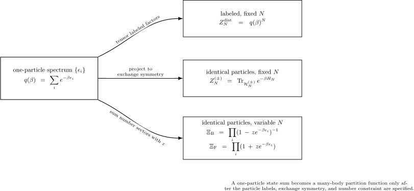
The same one-particle spectrum leads to different many-body partition functions depending on the Hilbert space and number constraint. Exchange symmetry and the sum over particle-number sectors are structural choices, not optional correction factors.

Distinguishable Noninteracting Particles

For $N$ labeled, noninteracting particles,

$$\mathcal H_{\mathrm{dist}} = \mathfrak h^{\otimes N},$$

and

$$H_N = \sum_{a=1}^{N} h_a.$$

The partition function factorizes:

$$Z_N^{\mathrm{dist}} = q(\beta)^N.$$

This formula counts permutations of one-particle occupations as distinct labeled states.

Identical Bosons and Fermions

For identical particles, the trace is restricted to the symmetric or antisymmetric subspace:

$$Z_N^{(\pm)} = \operatorname{Tr}_{\mathcal H_N^{(\pm)}} e^{-\beta H_N}.$$

The plus sign denotes bosons and the minus sign fermions. In general,

$$Z_N^{(\pm)} \neq q^N.$$

For noninteracting identical particles, an exact recurrence is

$$Z_N^{(\eta)} = \frac{1}{N} \sum_{\ell=1}^{N} \eta^{\ell-1} q(\ell\beta) Z_{N-\ell}^{(\eta)},$$

with

$$Z_0^{(\eta)}=1, \qquad \eta= \begin{cases} +1,&\text{bosons},\\ -1,&\text{fermions}. \end{cases}$$

The terms with $\ell>1$ are exchange corrections.

Maxwell–Boltzmann Limit

In the dilute, nondegenerate regime, exchange corrections become small and the identical-particle canonical partition function approaches

$$Z_N^{\mathrm{MB}} \simeq \frac{ q(\beta)^N }{ N! }.$$

The factor $1/N!$ prevents classical overcounting of particle labels. This is an approximation to the quantum bosonic or fermionic result, not an exact formula at arbitrary density.

Classical Limit of Quantum Statistics derives the controlling parameter $n\lambda_T^d/g$, the low-fugacity cycle expansion, and the leading Bose and Fermi virial corrections.

Noninteracting Modes in Fock Space

Suppose

$$H-\mu N = \sum_i (\epsilon_i-\mu)n_i.$$

The grand partition function factorizes over modes.

For bosons,

$$\begin{aligned} \Xi_{\mathrm B} &= \prod_i \sum_{n_i=0}^{\infty} \left( ze^{-\beta\epsilon_i} \right)^{n_i} \\ &= \prod_i \frac{1}{ 1-ze^{-\beta\epsilon_i} }, \end{aligned}$$

provided

$$\left| ze^{-\beta\epsilon_i} \right| < 1$$

for every mode.

For fermions,

$$\begin{aligned} \Xi_{\mathrm F} &= \prod_i \sum_{n_i=0}^{1} \left( ze^{-\beta\epsilon_i} \right)^{n_i} \\ &= \prod_i \left( 1+ze^{-\beta\epsilon_i} \right). \end{aligned}$$

Taking logarithms turns products into sums:

$$\ln\Xi_{\mathrm B} = -\sum_i \ln \left( 1-ze^{-\beta\epsilon_i} \right),$$

and

$$\ln\Xi_{\mathrm F} = \sum_i \ln \left( 1+ze^{-\beta\epsilon_i} \right).$$

Example: Two One-Particle Levels

Let

$$\epsilon_0=0, \qquad \epsilon_1=\Delta,$$

and define

$$x \equiv e^{-\beta\Delta}.$$

The one-particle partition function is

$$q = 1+x.$$

Two distinguishable particles

For two labeled particles,

$$Z_2^{\mathrm{dist}} = q^2 = 1+2x+x^2.$$

The coefficient $2x$ counts which labeled particle occupies the excited level.

Two identical bosons

The allowed occupation states are

$$(n_0,n_1) = (2,0),(1,1),(0,2).$$

Therefore

$$Z_2^{\mathrm B} = 1+x+x^2.$$

Two identical spinless fermions

Pauli exclusion allows only

$$(n_0,n_1) = (1,1).$$

Hence

$$Z_2^{\mathrm F} = x.$$

The three answers differ despite sharing the same one-particle spectrum.

Density-of-States Representation

Define

$$\omega(E) = \operatorname{Tr} \delta(E-H).$$

Then

$$Z(\beta) = \int dE\, \omega(E)e^{-\beta E}.$$

The partition function is the Laplace transform of the density of states.

For a discrete spectrum,

$$\omega(E) = \sum_a g_a\delta(E-E_a),$$

and the integral reduces to the spectral sum.

Formally, the inverse transform is

$$\omega(E) = \frac{1}{2\pi i} \int_{c-i\infty}^{c+i\infty} d\beta\, e^{\beta E}Z(\beta),$$

where the vertical contour lies in a domain of convergence. Inverse Laplace transforms are often numerically ill-conditioned; formal invertibility does not guarantee stable reconstruction from noisy data.

Microcanonical and Canonical Information

If

$$\omega(E) \sim \exp \left[ \frac{S(E)}{k_{\mathrm B}} \right],$$

then

$$Z(\beta) \sim \int dE\, \exp \left[ \frac{S(E)}{k_{\mathrm B}} -\beta E \right].$$

In a regular thermodynamic limit, the dominant energy satisfies

$$\frac{1}{k_{\mathrm B}} \frac{\partial S}{\partial E} = \beta.$$

Thus the partition function packages microcanonical state counting into a fixed-temperature generating object. The Microcanonical Ensemble page owns shell definitions and entropy conventions.

High-Temperature Expansion

In finite dimension,

$$e^{-\beta H} = \mathbb I -\beta H +\frac{\beta^2}{2}H^2 +O(\beta^3).$$

Therefore

$$Z(\beta) = d -\beta\operatorname{Tr}H +\frac{\beta^2}{2} \operatorname{Tr}H^2 +O(\beta^3),$$

where

$$d = \dim\mathcal H.$$

As $\beta\to0$,

$$\rho_\beta \longrightarrow \frac{\mathbb I}{d}.$$

In infinite dimension, this expansion need not define a trace because $Z(0)$ may diverge.

Low-Temperature Expansion

Let the ground energy be $E_0$ with degeneracy $g_0$, and let the next distinct energy be

$$E_1 = E_0+\Delta.$$

Then

$$Z(\beta) = e^{-\beta E_0} \left[ g_0 +g_1e^{-\beta\Delta} +\cdots \right].$$

At large positive $\beta$,

$$\ln Z = -\beta E_0 +\ln g_0 +O \left( e^{-\beta\Delta} \right).$$

The leading exponential reveals the ground energy, while the constant term reveals its degeneracy.

Finite Systems and Analyticity

For a finite spectrum,

$$Z(\beta) = \sum_a g_ae^{-\beta E_a}$$

is analytic for finite real $\beta$ and strictly positive there. Consequently,

$$\ln Z(\beta)$$

has no real-axis singularity at finite system size.

Sharp thermodynamic phase transitions require a limit in which system size diverges. In the complex plane, finite-system partition functions can have zeros. Families of such zeros can approach the physical real axis in a thermodynamic limit, producing nonanalytic bulk free energies.

Imaginary-Time Representation

The trace

$$Z = \operatorname{Tr} e^{-\beta H}$$

is an evolution trace over imaginary time of length

$$\beta\hbar.$$

For

$$H = \frac{p^2}{2m} +V(q),$$

the Trotter product divides the interval into $M$ slices. In the limit,

$$Z = \int_{q(\beta\hbar)=q(0)} \mathcal Dq\, e^{-S_{\mathrm E}[q]/\hbar},$$

with Euclidean action

$$S_{\mathrm E}[q] = \int_0^{\beta\hbar} d\tau \left[ \frac{m}{2} \left( \frac{dq}{d\tau} \right)^2 +V(q) \right].$$

The trace imposes periodic endpoint identification on coordinate paths.

This formula is a preview. Finite-Temperature QM Overview places the thermal trace in the wider KMS, Matsubara, spectral, and path-integral toolkit. Path Integrals for Statistical Mechanics develops the cyclic measure, normalization, exchange sectors, ring-polymer representation, and thermal oscillator determinant. Euclidean and Imaginary-Time Path Integrals retains the open-kernel and Wick-rotation construction.

Identical Particles in the Path Integral

For $N$ identical particles, the trace over symmetric or antisymmetric states can be represented schematically as

$$Z_N^{(\pm)} = \frac{1}{N!} \sum_{P\in S_N} (\pm1)^P \int dq\, \langle q| e^{-\beta H} |Pq\rangle.$$

Bosons sum permutations with positive sign. Fermions include permutation parity.

In coherent-state thermal path integrals, bosonic fields are periodic and fermionic Grassmann fields are antiperiodic in imaginary time. Coherent-State Path Integrals Preview derives these conditions from the trace and checks the corresponding Gaussian determinants. The distinction from first-quantized permutation closure is made explicit in Path Integrals for Statistical Mechanics.

Numerical Evaluation

Log-sum-exp stabilization

Directly summing

$$Z = \sum_a g_ae^{-\beta E_a}$$

can underflow at low temperature. Let $E_{\min}$ be the smallest retained energy. Then

$$\ln Z = -\beta E_{\min} +\ln \sum_a g_a e^{-\beta(E_a-E_{\min})}.$$

Every exponential in the remaining sum is at most one for $\beta>0$.

Work with logarithms

For independent modes or large lattices, compute $\ln Z$ or $\ln\Xi$ directly rather than forming exponentially large products.

For example,

$$\ln\Xi_{\mathrm F} = \sum_i \ln \left( 1+ze^{-\beta\epsilon_i} \right)$$

is more stable than multiplying all factors.

Check truncation

If a spectral sum is truncated, vary the energy cutoff until $\ln Z$ and target observables are stable. A cutoff adequate at low temperature may fail as temperature increases.

Respect sectors

Compute traces in the intended Hilbert space. A full-space trace can differ exponentially from a fixed-charge or fixed-symmetry trace.

Validate limits

Check:

$$\beta\to0, \qquad \beta\to+\infty,$$

known noninteracting limits, and exact small-system results.

Canonical Boundaries

This page owns:

• basis-independent trace and spectral-sum definitions;
• convergence and trace-class conditions;
• moment, cumulant, source, and number-generating interpretations;
• exact factorization criteria;
• the distinction among one-particle, distinguishable-particle, bosonic, fermionic, canonical, and grand partition functions;
• density-of-states transforms;
• high- and low-temperature asymptotics;
• imaginary-time trace and path-integral preview;
• numerical stabilization.

Other pages own:

• fixed-$T,N,V$ free energies, energy fluctuations, and reservoir interpretation: Canonical Ensemble;
• fixed-$T,\mu,V$ thermodynamics, convergence in particle-number sectors, and compressibility: Grand-Canonical Ensemble;
• equilibrium static response, ensemble dependence, and Kubo–Mori covariance: Fluctuations and Susceptibilities;
• the regime and accuracy of the Maxwell–Boltzmann approximation: Classical Limit of Quantum Statistics;
• energy shells and entropy derivatives: Microcanonical Ensemble;
• natural variables and Legendre transforms among potentials: Thermodynamic Potentials;
• Bose–Einstein and Fermi–Dirac occupations: Quantum Statistics and Ideal Gases;
• full path-integral derivations: Quantum Dynamics;
• compact lookup identities: Ensemble Formula Sheet.

Common Mistakes

Forgetting the trace space

$\operatorname{Tr}_{\mathcal H_N}$ and $\operatorname{Tr}_{\mathcal F}$ define different ensembles.

Dropping degeneracies

An energy value with degeneracy $g_a$ contributes

$$g_ae^{-\beta E_a}.$$

Calling the one-particle sum the many-body partition function

$q(\beta)$ becomes $q^N$ only for labeled noninteracting particles. Exchange symmetry changes the state count.

Dividing by the factorial outside its regime

$q^N/N!$ is the Maxwell–Boltzmann approximation for dilute identical particles, not the exact Bose or Fermi answer at arbitrary density.

Factoring an interacting trace

Independent terms and a tensor-product trace are required for $Z_{AB}=Z_AZ_B$.

Ignoring convergence

A formal trace that diverges does not normalize a density operator.

Holding the wrong variable fixed

Fixed fugacity, fixed $\alpha=\beta\mu$, and fixed chemical potential are not interchangeable under $\beta$ derivatives.

Replacing quantum susceptibility by an ordinary variance

For noncommuting observables, second source derivatives generate imaginary-time correlations.

Evaluating large products directly

Use logarithms and shifted energies to avoid overflow and underflow.

Exercises

Basis independence

Let $U$ be unitary. Show that

$$\operatorname{Tr} e^{-\beta UHU^\dagger} = \operatorname{Tr} e^{-\beta H}.$$

Solution

Functional calculus gives

$$e^{-\beta UHU^\dagger} = Ue^{-\beta H}U^\dagger.$$

Using cyclicity,

$$\begin{aligned} \operatorname{Tr} e^{-\beta UHU^\dagger} &= \operatorname{Tr} \left( Ue^{-\beta H}U^\dagger \right) \\ &= \operatorname{Tr} \left( U^\dagger Ue^{-\beta H} \right) \\ &= \operatorname{Tr} e^{-\beta H}. \end{aligned}$$

The partition function depends on the spectrum with multiplicity, not on the chosen basis.

Energy-shift invariance

For $H'=H+C\mathbb I$, derive $Z'$, $\rho'$, and $F'$.

Solution

Because $C\mathbb I$ commutes with $H$,

$$e^{-\beta H'} = e^{-\beta C} e^{-\beta H}.$$

Therefore

$$Z' = e^{-\beta C}Z.$$

The normalized state is

$$\rho' = \frac{ e^{-\beta C}e^{-\beta H} }{ e^{-\beta C}Z } = \rho.$$

Finally,

$$\begin{aligned} F' &= -k_{\mathrm B}T\ln Z' \\ &= -k_{\mathrm B}T \left( -\beta C+\ln Z \right) \\ &= C+F. \end{aligned}$$

Energy cumulants

Starting from

$$K_H(t) = \ln Z(\beta-t) -\ln Z(\beta),$$

show that the first two cumulants are the mean and variance of $H$.

Solution

The first derivative at $t=0$ is

$$\left. \frac{\partial K_H}{\partial t} \right|_{t=0} = -\frac{\partial\ln Z}{\partial\beta} = \langle H\rangle.$$

The second derivative is

$$\left. \frac{\partial^2K_H}{\partial t^2} \right|_{t=0} = \frac{\partial^2\ln Z}{\partial\beta^2}.$$

Direct differentiation gives

$$\frac{\partial^2\ln Z}{\partial\beta^2} = \langle H^2\rangle -\langle H\rangle^2.$$

Hence

$$\kappa_1(H) = \langle H\rangle, \qquad \kappa_2(H) = \operatorname{Var}(H).$$

Two particles in two levels

For one-particle energies $0$ and $\Delta$, compute the two-particle partition function for distinguishable particles, identical bosons, and identical spinless fermions.

Solution

Set

$$x=e^{-\beta\Delta}.$$

For labeled particles,

$$Z_2^{\mathrm{dist}} = (1+x)^2 = 1+2x+x^2.$$

For bosons, the occupations $(2,0)$, $(1,1)$, and $(0,2)$ have energies $0$, $\Delta$, and $2\Delta$, so

$$Z_2^{\mathrm B} = 1+x+x^2.$$

For two spinless fermions, both available orbitals must be occupied, giving total energy $\Delta$:

$$Z_2^{\mathrm F} = x.$$

Recover fixed-number sectors

For two fermionic modes with one-particle energies $\epsilon_1$ and $\epsilon_2$, expand

$$\Xi = \left( 1+ze^{-\beta\epsilon_1} \right) \left( 1+ze^{-\beta\epsilon_2} \right)$$

and identify $Z_0$, $Z_1$, and $Z_2$.

Solution

Expanding,

$$\begin{aligned} \Xi ={}& 1 \\ &+ z \left( e^{-\beta\epsilon_1} +e^{-\beta\epsilon_2} \right) \\ &+ z^2 e^{-\beta(\epsilon_1+\epsilon_2)}. \end{aligned}$$

Comparing with

$$\Xi = \sum_{N=0}^{2} z^NZ_N$$

gives

$$Z_0=1,$$ $$Z_1 = e^{-\beta\epsilon_1} +e^{-\beta\epsilon_2},$$

and

$$Z_2 = e^{-\beta(\epsilon_1+\epsilon_2)}.$$

The $N=2$ sector has one state because Pauli exclusion forces both modes to be occupied.

Factorization test

Let

$$H = H_A\otimes\mathbb I_B +\mathbb I_A\otimes H_B +gV_{AB}.$$

For which value of $g$ does exact factorization follow immediately? Explain why commutation of $V_{AB}$ with the uncoupled Hamiltonian is not by itself enough to give $Z=Z_AZ_B$.

Solution

At

$$g=0,$$

the Hamiltonian is a sum of operators on independent tensor factors, so

$$Z_{AB} = Z_AZ_B.$$

If $g\neq0$ and $V_{AB}$ commutes with the uncoupled Hamiltonian, then

$$e^{-\beta H} = e^{-\beta H_A} \otimes e^{-\beta H_B} e^{-\beta gV_{AB}},$$

with the tensor factors understood on the full space. The extra operator $e^{-\beta gV_{AB}}$ generally couples the trace over $A$ and $B$, so its trace does not split into $Z_AZ_B$.

Commutation simplifies the exponential but does not remove the interaction or restore a product state count.

Cross-Links

• Statistical Ensembles Overview
• Microcanonical Ensemble
• Thermal Density Operators
• Canonical Ensemble
• Grand-Canonical Ensemble
• Thermodynamic Potentials
• Ensemble Equivalence
• Ensemble Formula Sheet
• Green Functions and Density of States
• Trace-Class and Hilbert–Schmidt Operators
• Tensor Products
• Fock Space and Occupation Number
• Quantum Statistics Overview
• Maxwell–Boltzmann Limit
• Bose–Einstein Statistics
• Fermi–Dirac Statistics
• Ideal Bose Gas
• Ideal Fermi Gas
• Euclidean and Imaginary-Time Path Integrals
• Statistical Mechanics Checklist

References

• R. K. Pathria and P. D. Beale, Statistical Mechanics, 4th ed., Elsevier (2021), chapters 3–8.
• K. Huang, Statistical Mechanics, 2nd ed., Wiley (1987), chapters 7–12.
• M. Kardar, Statistical Physics of Particles, Cambridge University Press (2007), chapters 2–6.
• L. D. Landau and E. M. Lifshitz, Statistical Physics, Part 1, 3rd ed., Butterworth–Heinemann (1980), sections 31–56.
• A. L. Fetter and J. D. Walecka, Quantum Theory of Many-Particle Systems, Dover (2003), chapters 1 and 2.
• R. P. Feynman and A. R. Hibbs, Quantum Mechanics and Path Integrals, emended ed., Dover (2010), chapters 2 and 10.
• H. Kleinert, Path Integrals in Quantum Mechanics, Statistics, Polymer Physics, and Financial Markets, 5th ed., World Scientific (2009), chapters 2 and 7.
• C. N. Yang and T. D. Lee, “Statistical Theory of Equations of State and Phase Transitions. I. Theory of Condensation”, Physical Review 87, 404–409 (1952).