Ideal Fermi Gas

The ideal Fermi gas is a system of noninteracting identical fermions. Its Hamiltonian is a sum of one-particle energies, yet its many-body ground state has a nonzero energy and pressure because Pauli exclusion forces particles to fill distinct modes.

For a uniform gas in a cubic box of volume $V=L^3$,

$$H = \sum_{\mathbf k,a} \epsilon_{\mathbf k} c_{\mathbf k a}^\dagger c_{\mathbf k a}, \qquad \epsilon_{\mathbf k} = \frac{\hbar^2k^2}{2m}.$$

The index $a=1,\ldots,g$ labels independent spin or internal modes. The number operator is

$$N = \sum_{\mathbf k,a} c_{\mathbf k a}^\dagger c_{\mathbf k a}.$$

The model is exactly solvable because every occupation number is conserved and satisfies

$$n_{\mathbf k a} \in \{0,1\}.$$

The ideal gas is the reference point for electrons in simple metals, cold fermionic atoms, nuclear and astrophysical estimates, Fermi-liquid theory, and any calculation organized around a filled Fermi sea.

This page owns the full uniform-gas thermodynamic derivation. The Ideal Fermi Gas dossier owns the compact baseline record, quantity-specific exactness audit, finite-volume checks, model variants, and numerical benchmark handoff.

Unless stated otherwise, this page uses:

• three spatial dimensions;
• a uniform cubic box;
• periodic boundary conditions;
• nonrelativistic dispersion;
• internal degeneracy $g$;
• fixed number density $n=N/V$;
• the thermodynamic limit.

Physical Setup

Periodic boundary conditions give one-particle modes

$$\phi_{\mathbf k a}(\mathbf r) = \frac{1}{\sqrt V} e^{i\mathbf k\cdot\mathbf r} \chi_a,$$

with

$$\mathbf k = \frac{2\pi}{L} \mathbf n, \qquad \mathbf n \in \mathbb Z^3.$$

The many-body eigenstates are fermionic occupation-number states

$$\lvert\{n_{\mathbf k a}\}\rangle.$$

Their particle number and energy are

$$N = \sum_{\mathbf k,a} n_{\mathbf k a},$$

and

$$E = \sum_{\mathbf k,a} \epsilon_{\mathbf k} n_{\mathbf k a}.$$

No potential energy appears because the particles do not interact. The nonzero ground-state energy is entirely kinetic and statistical in origin.

Grand Partition Function

Define

$$z \equiv e^{\beta\mu}, \qquad \beta = \frac{1}{k_{\mathrm B}T}.$$

One fermionic mode contributes

$$\xi_{\mathbf k a} = 1+ze^{-\beta\epsilon_{\mathbf k}}.$$

Therefore

$$\Xi = \prod_{\mathbf k,a} \left( 1+ze^{-\beta\epsilon_{\mathbf k}} \right),$$

and

$$\ln\Xi = \sum_{\mathbf k,a} \ln \left( 1+ze^{-\beta\epsilon_{\mathbf k}} \right).$$

Unlike the bosonic product, every finite fermionic mode factor is finite for every finite real $\mu$. Infinite-volume expressions still require a thermodynamic limit and a controlled density of states.

The mode occupation is

$$\overline n_{\mathbf k a} = \frac{1}{ z^{-1}e^{\beta\epsilon_{\mathbf k}}+1 }.$$

Momentum-Space State Counting

One momentum mode per internal state occupies volume

$$\left( \frac{2\pi}{L} \right)^3$$

in $\mathbf k$-space. Including all $g$ internal modes, the number of one-particle states with magnitude below $k$ is

$$\mathcal N(k) = g \frac{V}{(2\pi)^3} \frac{4\pi k^3}{3} = \frac{gVk^3}{6\pi^2}.$$

At zero temperature, the lowest $N$ modes are occupied. For the isotropic dispersion, they fill a sphere of radius $k_{\mathrm F}$ in momentum space.

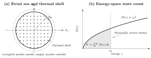
At $T=0$, every complete one-particle mode inside the Fermi sphere is occupied and every mode outside is empty. The same state count is the area under $D(\epsilon)$ up to $\epsilon_{\mathrm F}$; thermal excitations affect only a narrow shell near the boundary when $T\ll T_{\mathrm F}$.

Fermi Momentum

Equating the state count to the particle number gives

$$N = \frac{gVk_{\mathrm F}^3}{6\pi^2}.$$

Thus

$$n = \frac{gk_{\mathrm F}^3}{6\pi^2},$$

and

$$k_{\mathrm F} = \left( \frac{6\pi^2n}{g} \right)^{1/3}.$$

For spin-$1/2$ fermions with two equally populated internal states, $g=2$:

$$k_{\mathrm F} = \left( 3\pi^2n \right)^{1/3}.$$

The density $n$ here is the total density summed over internal states. Using the density per spin component in the same formula without adjusting $g$ double-counts the degeneracy.

Fermi Energy, Temperature, and Velocity

The Fermi energy is the one-particle energy at $k_{\mathrm F}$:

$$\epsilon_{\mathrm F} = \frac{\hbar^2k_{\mathrm F}^2}{2m}.$$

The Fermi temperature is

$$T_{\mathrm F} \equiv \frac{\epsilon_{\mathrm F}}{k_{\mathrm B}},$$

and the Fermi velocity is

$$v_{\mathrm F} = \frac{1}{\hbar} \left. \frac{d\epsilon_k}{dk} \right|_{k=k_{\mathrm F}} = \frac{\hbar k_{\mathrm F}}{m}.$$

These are density scales, not independent parameters. For the uniform ideal gas,

$$\epsilon_{\mathrm F} \propto n^{2/3}.$$

Three-Dimensional Density of States

Using

$$k = \frac{\sqrt{2m\epsilon}}{\hbar},$$

the integrated state count is

$$\mathcal N(\epsilon) = \frac{gV}{6\pi^2} \left( \frac{2m\epsilon}{\hbar^2} \right)^{3/2}.$$

The density of states is

$$D(\epsilon) = \frac{gV}{4\pi^2} \left( \frac{2m}{\hbar^2} \right)^{3/2} \sqrt\epsilon.$$

It includes the internal degeneracy $g$. If a quoted density of states is per spin or per component, $g$ must not be inserted again.

At the Fermi energy,

$$D(\epsilon_{\mathrm F}) = \frac{3N}{2\epsilon_{\mathrm F}}.$$

Per unit volume,

$$\frac{D(\epsilon_{\mathrm F})}{V} = \frac{3n}{2\epsilon_{\mathrm F}}.$$

The density of states near $\epsilon_{\mathrm F}$ controls low-temperature heat capacity, compressibility, and many weak-response coefficients.

Zero-Temperature Occupation

At fixed density, the chemical potential approaches the Fermi energy as $T\to0$:

$$\mu(0) = \epsilon_{\mathrm F}.$$

The occupation becomes

$$\overline n_{\mathbf k a} = \Theta \left( k_{\mathrm F}-k \right),$$

away from the boundary. Equivalently,

$$\overline n(\epsilon) = \Theta \left( \epsilon_{\mathrm F}-\epsilon \right).$$

The filled region is the Fermi sea. The sphere $k=k_{\mathrm F}$ is the Fermi surface of this isotropic continuum model.

The Fermi surface is a surface in momentum space, not a physical boundary in the box.

Ground-State Energy

At zero temperature,

$$U_0 = \int_0^{\epsilon_{\mathrm F}} d\epsilon\, D(\epsilon)\epsilon.$$

Since $D(\epsilon)\propto\sqrt\epsilon$,

$$U_0 = \frac{3}{5} N\epsilon_{\mathrm F}.$$

Thus the mean energy per particle is

$$\frac{U_0}{N} = \frac{3}{5} \epsilon_{\mathrm F}.$$

The ground-state energy is nonzero even without interactions. Pauli exclusion forces particles into modes with increasing kinetic energy.

Degeneracy Pressure

For a nonrelativistic quadratic dispersion in three dimensions,

$$P = \frac{2U}{3V}.$$

At zero temperature,

$$P_0 = \frac{2}{5} n\epsilon_{\mathrm F}.$$

Because $\epsilon_{\mathrm F}\propto n^{2/3}$,

$$P_0 \propto n^{5/3}.$$

This pressure persists at $T=0$. It is called degeneracy pressure and follows from the density dependence of the allowed fermionic kinetic states, not from thermal motion or a pairwise repulsive force.

Zero-Temperature Compressibility

Differentiating

$$P_0 = \frac{2}{5}n\epsilon_{\mathrm F}$$

at fixed particle species gives

$$\frac{dP_0}{dn} = \frac{2}{3} \epsilon_{\mathrm F}.$$

The zero-temperature compressibility is therefore

$$\kappa_0 = \frac{1}{n} \left( \frac{\partial n}{\partial P} \right)_{T=0} = \frac{3}{2n\epsilon_{\mathrm F}}.$$

Susceptibilities distinguishes this isothermal normalization from $\partial n/\partial\mu$ and from the retarded density response, including the required order of limits.

Equivalently,

$$\left( \frac{\partial n}{\partial\mu} \right)_{T=0} = \frac{D(\epsilon_{\mathrm F})}{V} = \frac{3n}{2\epsilon_{\mathrm F}}.$$

Finite-Temperature Number and Energy

At positive temperature,

$$N = \int_0^\infty d\epsilon\, D(\epsilon) \frac{1}{ e^{\beta(\epsilon-\mu)}+1 },$$

and

$$U = \int_0^\infty d\epsilon\, D(\epsilon) \frac{\epsilon}{ e^{\beta(\epsilon-\mu)}+1 }.$$

At fixed $n$, the number equation determines $\mu(T)$. Treating $\mu$ as fixed at $\epsilon_{\mathrm F}$ for all temperatures violates the fixed-density constraint.

The pressure remains related to energy by

$$P = \frac{2U}{3V}$$

for the uniform ideal gas with quadratic dispersion at every temperature.

Thermal Wavelength and Polylogarithm Form

Use the thermal wavelength

$$\lambda_T = \sqrt{ \frac{2\pi\hbar^2}{mk_{\mathrm B}T} }.$$

The continuum grand partition function is

$$\ln\Xi = - \frac{gV}{\lambda_T^3} \operatorname{Li}_{5/2}(-z).$$

The number equation becomes

$$n = - \frac{g}{\lambda_T^3} \operatorname{Li}_{3/2}(-z),$$

and the pressure is

$$P = - \frac{gk_{\mathrm B}T}{\lambda_T^3} \operatorname{Li}_{5/2}(-z).$$

The polylogarithms are negative for $z>0$ in these combinations, so $n$ and $P$ are positive.

Some references define normalized Fermi integrals with indices shifted by one. Stating the polylogarithm form prevents an otherwise common index-convention ambiguity.

Classical Dilute Limit

For $z\ll1$,

$$-\operatorname{Li}_s(-z) = z - \frac{z^2}{2^s} + O(z^3).$$

Define the phase-space density per internal state,

$$x \equiv \frac{n\lambda_T^3}{g}.$$

Then

$$x = z - \frac{z^2}{2^{3/2}} + O(z^3),$$

while

$$\frac{P\lambda_T^3}{ gk_{\mathrm B}T } = z - \frac{z^2}{2^{5/2}} + O(z^3).$$

Eliminating $z$ gives

$$\frac{P}{nk_{\mathrm B}T} = 1 + \frac{n\lambda_T^3}{ 2^{5/2}g } + O \left[ \left( \frac{n\lambda_T^3}{g} \right)^2 \right].$$

The positive correction reflects Pauli exclusion. It is a statistical contribution, not a physical repulsive potential.

Degenerate Regime

The gas is quantum degenerate when

$$T \ll T_{\mathrm F}.$$

Most modes far below $\epsilon_{\mathrm F}$ remain occupied, and most modes far above remain empty. Only states within an energy window of order $k_{\mathrm B}T$ around the Fermi energy change occupation appreciably.

The fraction of particles participating in thermal excitations is therefore of order

$$\frac{T}{T_{\mathrm F}},$$

not order one. This is why the low-temperature heat capacity is linear in $T$ rather than approaching the classical value $3Nk_{\mathrm B}/2$.

Sommerfeld Expansion Preview

For a smooth function $\varphi(\epsilon)$ and $k_{\mathrm B}T\ll\mu$,

$$\begin{aligned} \int_0^\infty d\epsilon\, \varphi(\epsilon) f_{\mathrm F}(\epsilon) ={}& \int_0^\mu d\epsilon\, \varphi(\epsilon) \\ &+ \frac{\pi^2}{6} (k_{\mathrm B}T)^2 \varphi'(\mu) \\ &+ O(T^4). \end{aligned}$$

This is the leading Sommerfeld expansion. Its canonical page owns the derivation, higher terms, regularity conditions, and endpoint cautions. Here it is used only to state the ideal-gas low-temperature results.

Low-Temperature Chemical Potential

At fixed density in the three-dimensional ideal gas,

$$\mu(T) = \epsilon_{\mathrm F} \left[ 1 - \frac{\pi^2}{12} \left( \frac{T}{T_{\mathrm F}} \right)^2 + O \left( \frac{T^4}{T_{\mathrm F}^4} \right) \right].$$

The chemical potential decreases quadratically from $\epsilon_{\mathrm F}$ at low temperature.

This coefficient depends on the energy dependence of the three-dimensional free-particle density of states. It is not the same for every band structure or dimension.

Low-Temperature Energy and Heat Capacity

At fixed density,

$$\frac{U}{N} = \frac{3}{5} \epsilon_{\mathrm F} \left[ 1 + \frac{5\pi^2}{12} \left( \frac{T}{T_{\mathrm F}} \right)^2 + O \left( \frac{T^4}{T_{\mathrm F}^4} \right) \right].$$

Differentiating gives

$$\frac{C_V}{N} = \frac{\pi^2}{2} k_{\mathrm B} \frac{T}{T_{\mathrm F}} + O \left( \frac{T^3}{T_{\mathrm F}^3} \right).$$

The entropy has the same leading coefficient:

$$\frac{S}{N} = \frac{\pi^2}{2} k_{\mathrm B} \frac{T}{T_{\mathrm F}} + O \left( \frac{T^3}{T_{\mathrm F}^3} \right).$$

Only the thin thermally active shell near the Fermi surface contributes at low temperature.

Low-Temperature Pressure

Using $P=2U/(3V)$,

$$\begin{aligned} P ={}& \frac{2}{5} n\epsilon_{\mathrm F} \Biggl[ 1 + \frac{5\pi^2}{12} \left( \frac{T}{T_{\mathrm F}} \right)^2 \\ &\qquad + O \left( \frac{T^4}{T_{\mathrm F}^4} \right) \Biggr]. \end{aligned}$$

Thermal pressure is a correction to the already nonzero degeneracy pressure.

Number Fluctuations

For independent grand-canonical modes,

$$\operatorname{Var}(N) = \sum_{\mathbf k,a} \overline n_{\mathbf k a} \left( 1- \overline n_{\mathbf k a} \right).$$

At zero temperature, modes away from the Fermi surface have occupations zero or one and therefore no mode-number variance. At low temperature, fluctuations are concentrated near $\epsilon_{\mathrm F}$.

The fluctuation–response relation is

$$\left( \frac{\partial\overline N}{\partial\mu} \right)_{T,V} = \beta \operatorname{Var}(N).$$

A fixed-$N$ canonical gas has no total-number fluctuation and has correlations among mode occupations. Ensemble equivalence for bulk thermodynamics does not make every global fluctuation identical.

Pauli Blocking

Scattering into a final fermionic mode carries an availability factor

$$1-f_{\mathrm F}(\epsilon_f).$$

At low temperature, modes deep inside the Fermi sea are already occupied and unavailable as final states. This suppresses scattering and relaxation channels whose final states would lie below the Fermi surface.

Pauli blocking follows from antisymmetry. It should not be described as an additional force between particles.

Finite Size and Shell Structure

In a finite box, the allowed momenta are discrete. The ground state fills complete shells of equal $k^2$ when possible. If the last shell is partially filled, the ground state can be degenerate.

Consequences include:

• stepwise changes in addition energy;
• shell-dependent chemical potentials;
• finite-size oscillations in energy and response;
• sensitivity to boundary conditions;
• no perfectly sharp continuum Fermi surface.

The continuum formulas require many occupied modes and observables coarse enough not to resolve individual level spacings. Finite-Size Effects gives the general shell, parity, boundary, and resolution audit; this page retains the Fermi-gas thermodynamics.

Example: Electrons in a Simple Metal

For free electrons, $g=2$ and

$$k_{\mathrm F} = (3\pi^2n)^{1/3}.$$

The ideal gas explains the existence of a Fermi energy, degeneracy pressure, and a heat capacity much smaller than the classical prediction at ordinary temperatures when $T\ll T_{\mathrm F}$.

Real electrons move in a crystal potential and interact. Band dispersions, effective masses, multiple Fermi-surface sheets, electron–electron interactions, and phonons modify the free-gas picture. Material-specific bands and transport belong to Quantum Matter.

Example: Ultracold Fermionic Atoms

For a dilute gas of neutral fermionic atoms, the internal-state degeneracy and population balance are experimentally controlled. In the weakly interacting limit, the ideal gas supplies $k_{\mathrm F}$, $\epsilon_{\mathrm F}$, $T_{\mathrm F}$, and the baseline density profile.

Interaction strength is often compared with the Fermi scale. Near a Feshbach resonance, pairing and strong correlations make the ideal model insufficient, but its Fermi units remain useful reference scales.

Example: Nuclear and Astrophysical Matter

Neutrons, protons, and electrons are fermions, so ideal-gas degeneracy pressure provides a first estimate for dense matter.

The nonrelativistic formula

$$P_0 = \frac{2}{5}n\epsilon_{\mathrm F}$$

fails when momenta become relativistic or when strong interactions dominate. White-dwarf electrons can require a relativistic Fermi gas, while neutron-star matter requires nuclear interactions, relativity, composition constraints, and gravity.

The ideal nonrelativistic gas is an organizing baseline, not a realistic equation of state for compact stars.

Other Dimensions and Dispersions

The numerical coefficients above are specific to

$$d = 3, \qquad \epsilon_k = \frac{\hbar^2k^2}{2m}.$$

In another dimension, the $k$-space volume and density of states change. On a lattice, the Fermi sea follows a band dispersion and need not be spherical. For anisotropic effective masses, constant-energy surfaces are ellipsoids rather than spheres.

The robust procedure is:

1. Specify the dispersion and degeneracies.
2. Count states below the chemical potential.
3. Integrate the Fermi–Dirac occupations.

What the Ideal Model Omits

The ideal Fermi gas omits:

• interparticle interactions;
• self-energy shifts and finite lifetimes;
• pairing and superconductivity;
• screening and collective modes;
• crystal bands and lattice geometry;
• disorder;
• relativistic dispersion;
• collision rates and equilibration mechanisms.

An interacting Fermi liquid may retain a Fermi surface and quasiparticles, but its effective mass, compressibility, heat capacity, and response contain interaction corrections. Random Phase Approximation uses this ideal gas as the reference polarization and resums induced density feedback to describe screening and collective charge modes. A strongly correlated system may not admit a simple quasiparticle description at all.

Canonical Boundaries

This page owns:

• the uniform three-dimensional nonrelativistic ideal Fermi gas;
• momentum-space state counting with internal degeneracy $g$;
• $k_{\mathrm F}$, $\epsilon_{\mathrm F}$, $T_{\mathrm F}$, and $v_{\mathrm F}$ in this model;
• the density of states and filled Fermi sea;
• zero-temperature energy, pressure, and compressibility;
• finite-temperature number, pressure, and energy integrals;
• leading low-temperature thermodynamics;
• finite-size, dimensional, relativistic, and interaction limitations.

Other pages own:

• the one-mode Fermi–Dirac distribution and thermal window: Fermi–Dirac Statistics;
• the $T\gg T_{\mathrm F}$ Maxwell–Boltzmann criterion and leading exchange correction: Classical Limit of Quantum Statistics;
• a focused treatment of $T\ll T_{\mathrm F}$ and physical applications: Degenerate Fermi Gas;
• dimension-by-dimension reference formulas: Fermi Momentum and Fermi Energy;
• generic Fermi-surface geometry and low-energy kinematics: Fermi Surface;
• the general low-temperature asymptotic method: Sommerfeld Expansion;
• Fermi surfaces in bands and materials: Quantum Matter;
• interacting quasiparticles and Fermi-liquid theory: Quasiparticles and Collective Modes;
• direct screening and collective density response around the ideal reference: Random Phase Approximation;
• relativistic degenerate matter: Relativistic QM and QFT.org.

Common Mistakes

• Forgetting the internal degeneracy factor $g$ in the state count.
• Counting $g$ twice when the density of states already includes it.
• Using total density in a per-component formula, or vice versa.
• Treating the Fermi surface as a surface in real space.
• Calling degeneracy pressure a thermal pressure or a new repulsive force.
• Setting the zero-temperature energy to zero because the particles do not interact.
• Assuming $\mu=\epsilon_{\mathrm F}$ at every temperature.
• Applying the three-dimensional free-particle density of states to a lattice band or trap.
• Using Maxwell–Boltzmann statistics when $T\ll T_{\mathrm F}$.
• Assigning the classical heat capacity $3Nk_{\mathrm B}/2$ to a degenerate Fermi gas.
• Applying Sommerfeld coefficients without checking the density of states and fixed variables.
• Using the nonrelativistic pressure for ultrarelativistic fermions.
• Treating an interacting electron, neutron, or cold-atom system as ideal without a controlled approximation.

Exercises

Count the Fermi sphere

Derive

$$k_{\mathrm F} = \left( \frac{6\pi^2n}{g} \right)^{1/3}$$

for a three-dimensional periodic box.

Solution

Each momentum state occupies volume $(2\pi/L)^3$ in $\mathbf k$-space. Including $g$ internal modes, the number of states inside a sphere of radius $k_{\mathrm F}$ is

$$\begin{aligned} N &= g \frac{V}{(2\pi)^3} \frac{4\pi k_{\mathrm F}^3}{3} \\ &= \frac{gVk_{\mathrm F}^3}{6\pi^2}. \end{aligned}$$

Dividing by $V$ gives

$$n = \frac{gk_{\mathrm F}^3}{6\pi^2}.$$

Solving for $k_{\mathrm F}$ gives the stated expression.

Derive the ground-state energy and pressure

Show that

$$U_0 = \frac{3}{5}N\epsilon_{\mathrm F}$$

and

$$P_0 = \frac{2}{5}n\epsilon_{\mathrm F}.$$

Solution

Write the density of states as

$$D(\epsilon) = A\epsilon^{1/2}.$$

The number is

$$N = A \int_0^{\epsilon_{\mathrm F}} d\epsilon\, \epsilon^{1/2} = \frac{2A}{3} \epsilon_{\mathrm F}^{3/2}.$$

The energy is

$$\begin{aligned} U_0 &= A \int_0^{\epsilon_{\mathrm F}} d\epsilon\, \epsilon^{3/2} \\ &= \frac{2A}{5} \epsilon_{\mathrm F}^{5/2} \\ &= \frac{3}{5} N\epsilon_{\mathrm F}. \end{aligned}$$

For a quadratic dispersion in three dimensions,

$$P_0 = \frac{2U_0}{3V} = \frac{2}{5} n\epsilon_{\mathrm F}.$$

Relate the density of states to particle number

Show that

$$D(\epsilon_{\mathrm F}) = \frac{3N}{2\epsilon_{\mathrm F}}.$$

Solution

Since

$$D(\epsilon) = A\epsilon^{1/2},$$

the zero-temperature particle number is

$$\begin{aligned} N &= \int_0^{\epsilon_{\mathrm F}} d\epsilon\, D(\epsilon) \\ &= \frac{2A}{3} \epsilon_{\mathrm F}^{3/2}. \end{aligned}$$

But

$$D(\epsilon_{\mathrm F}) = A\epsilon_{\mathrm F}^{1/2}.$$

Eliminating $A$ gives

$$D(\epsilon_{\mathrm F}) = \frac{3N}{2\epsilon_{\mathrm F}}.$$

Recover the linear heat capacity

Use

$$\frac{U}{N} = \frac{3}{5} \epsilon_{\mathrm F} \left[ 1+ \frac{5\pi^2}{12} \left( \frac{T}{T_{\mathrm F}} \right)^2 \right]$$

to derive the leading low-temperature heat capacity at fixed $N$ and $V$.

Solution

The temperature-dependent energy correction is

$$\begin{aligned} \Delta U &= N \frac{3}{5} \epsilon_{\mathrm F} \frac{5\pi^2}{12} \frac{T^2}{T_{\mathrm F}^2} \\ &= N \frac{\pi^2}{4} \frac{k_{\mathrm B}^2T^2}{ \epsilon_{\mathrm F} }. \end{aligned}$$

Differentiating gives

$$\begin{aligned} C_V &= \left( \frac{\partial U}{\partial T} \right)_{N,V} \\ &= N \frac{\pi^2}{2} \frac{k_{\mathrm B}^2T}{ \epsilon_{\mathrm F} } \\ &= N \frac{\pi^2}{2} k_{\mathrm B} \frac{T}{T_{\mathrm F}}. \end{aligned}$$

Find the leading classical correction

Show that the dilute ideal Fermi gas obeys

$$\begin{aligned} \frac{P}{nk_{\mathrm B}T} ={}& 1 + \frac{n\lambda_T^3}{ 2^{5/2}g } \\ &+ O \left[ \left( \frac{n\lambda_T^3}{g} \right)^2 \right]. \end{aligned}$$

Solution

Let

$$x = \frac{n\lambda_T^3}{g}.$$

The number expansion is

$$x = z- \frac{z^2}{2^{3/2}} + O(z^3).$$

Inverting gives

$$z = x+ \frac{x^2}{2^{3/2}} + O(x^3).$$

The pressure expansion is

$$\frac{P\lambda_T^3}{ gk_{\mathrm B}T } = z- \frac{z^2}{2^{5/2}} + O(z^3).$$

Substitution yields

$$\frac{P\lambda_T^3}{ gk_{\mathrm B}T } = x+ \frac{x^2}{2^{5/2}} + O(x^3).$$

Dividing by $x$ gives the stated positive statistical correction.

Cross-Links

• Quantum Gas Formula Sheet
• Fermi Gas Formula Sheet
• Ideal Fermi Gas Model Dossier
• Quantum Statistics Overview
• Maxwell–Boltzmann Limit
• Fermi–Dirac Statistics
• Degenerate Fermi Gas
• Fermi Momentum and Fermi Energy
• Fermi Surface
• Green Functions in Many-Body QM
• Susceptibilities
• Ideal Bose Gas
• Benchmark Problems — the MB-B007 zero-temperature and Sommerfeld-coefficient contract.
• Grand-Canonical Ensemble
• Thermodynamic Limit
• Occupation-Number Representation
• Field Operators in Many-Body Models
• Ideal Fermi Gas Model Card
• Fermi–Dirac Distribution Formula Card
• Fermionic Fock Space
• Pauli Exclusion Principle
• Density of States: First Encounter

References

• R. K. Pathria and P. D. Beale, Statistical Mechanics, 3rd ed., Elsevier (2011).
• K. Huang, Statistical Mechanics, 2nd ed., Wiley (1987).
• M. Kardar, Statistical Physics of Particles, Cambridge University Press (2007).
• L. D. Landau and E. M. Lifshitz, Statistical Physics, Part 1, 3rd ed., Butterworth–Heinemann (1980).
• A. L. Fetter and J. D. Walecka, Quantum Theory of Many-Particle Systems, Dover (2003).
• N. W. Ashcroft and N. D. Mermin, Solid State Physics, Holt, Rinehart and Winston (1976).
• G. D. Mahan, Many-Particle Physics, 3rd ed., Springer (2000).
• S. Giorgini, L. P. Pitaevskii, and S. Stringari, “Theory of ultracold atomic Fermi gases,” Reviews of Modern Physics 80, 1215–1274 (2008).