Ideal Bose Gas

The ideal Bose gas is a system of noninteracting identical bosons. Its Hamiltonian is a sum of one-particle energies, but its thermodynamics is not classical because every mode can hold any nonnegative number of bosons.

For a uniform gas in a cubic box of volume $V=L^3$,

$$H = \sum_{\mathbf k} \epsilon_{\mathbf k} a_{\mathbf k}^\dagger a_{\mathbf k}, \qquad \epsilon_{\mathbf k} = \frac{\hbar^2k^2}{2m}.$$

The number operator is

$$N = \sum_{\mathbf k} a_{\mathbf k}^\dagger a_{\mathbf k}.$$

The model is exactly solvable because all number operators commute and the many-body eigenstates are occupation-number states. Its importance is disproportionate to its simplicity: it isolates the thermodynamic consequences of Bose statistics, supplies the reference point for weakly interacting gases, and shows how a macroscopic ground-mode occupation can emerge from a one-particle spectrum.

This page owns the full thermodynamic derivation. The Ideal Bose Gas dossier owns the compact baseline record, quantity-specific exactness audit, finite-volume checks, model variants, and numerical benchmark handoff.

Unless stated otherwise, this page uses:

• one spinless bosonic species;
• three spatial dimensions;
• a uniform cubic box;
• periodic boundary conditions;
• positive temperature;
• ground-state energy $\epsilon_0=0$;
• the thermodynamic limit at fixed density $n=N/V$.

Physical Setup

Periodic boundary conditions give normalized one-particle eigenfunctions

$$\phi_{\mathbf k}(\mathbf r) = \frac{1}{\sqrt V} e^{i\mathbf k\cdot\mathbf r},$$

with allowed wavevectors

$$\mathbf k = \frac{2\pi}{L} \mathbf n, \qquad \mathbf n \in \mathbb Z^3.$$

The lowest mode is $\mathbf k=\mathbf0$. Its energy is chosen to be zero:

$$\epsilon_{\mathbf0} = 0.$$

An occupation configuration

$$\lvert\{n_{\mathbf k}\}\rangle$$

has

$$n_{\mathbf k} = 0,1,2,\ldots,$$

total particle number

$$N = \sum_{\mathbf k} n_{\mathbf k},$$

and energy

$$E = \sum_{\mathbf k} \epsilon_{\mathbf k}n_{\mathbf k}.$$

The particles do not interact. All nonclassical thermodynamics comes from bosonic state counting and the density of one-particle levels.

Why the Ground Mode Must Be Separated

The excited levels become dense as $L\to\infty$, so their sum can be replaced by an energy integral. The ground state remains one distinguished mode and should be kept explicit:

$$N = N_0 + N_{\mathrm{ex}}.$$

Here

$$N_0 = \langle n_{\mathbf0}\rangle$$

is the ground-mode occupation, while $N_{\mathrm{ex}}$ sums all $\mathbf k\neq\mathbf0$ modes.

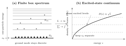
In a finite box the spectrum is discrete and the $\mathbf k=\mathbf0$ mode is unique. In the thermodynamic limit the excited levels become a continuum with $D(\epsilon)\propto\sqrt\epsilon$ in three dimensions, but the ground mode must remain separate when its occupation is macroscopic.

Replacing the entire spectrum by one continuum integral can erase the very mode whose macroscopic occupation defines ideal-gas condensation.

Grand Partition Function

Introduce the fugacity

$$z \equiv e^{\beta\mu}, \qquad \beta = \frac{1}{k_{\mathrm B}T}.$$

Because the ground energy is zero, convergence requires

$$0 < z < 1,$$

or equivalently

$$\mu < 0$$

for a finite grand-canonical system.

The mode factor is

$$\xi_{\mathbf k} = \frac{1}{ 1-ze^{-\beta\epsilon_{\mathbf k}} }.$$

Therefore

$$\Xi = \prod_{\mathbf k} \frac{1}{ 1-ze^{-\beta\epsilon_{\mathbf k}} },$$

and

$$\ln\Xi = - \sum_{\mathbf k} \ln \left( 1-ze^{-\beta\epsilon_{\mathbf k}} \right).$$

Separating the ground mode gives

$$\begin{aligned} \ln\Xi ={}& -\ln(1-z) \\ &- \sum_{\mathbf k\neq\mathbf0} \ln \left( 1-ze^{-\beta\epsilon_{\mathbf k}} \right). \end{aligned}$$

The first term is the exact ground-mode contribution. The second becomes extensive in the thermodynamic limit.

Mode Occupations and Number Equation

Every momentum mode has mean occupation

$$\overline n_{\mathbf k} = \frac{1}{ z^{-1}e^{\beta\epsilon_{\mathbf k}}-1 }.$$

For the ground mode,

$$N_0 = \frac{z}{1-z}.$$

The exact finite-volume number equation is

$$N = \frac{z}{1-z} + \sum_{\mathbf k\neq\mathbf0} \frac{1}{ z^{-1}e^{\beta\epsilon_{\mathbf k}}-1 }.$$

At fixed $N$, $V$, and $T$, this equation determines $z$ and therefore $\mu$.

The equation also exposes the two distinct ways to store particles: distribute them among excited modes, or accumulate them in the single ground mode as $z\to1^-$.

Counting One-Particle States

In a large periodic box, one momentum state occupies volume

$$\left( \frac{2\pi}{L} \right)^3$$

in $\mathbf k$-space. The number of spinless modes with magnitude below $k$ is

$$\mathcal N(k) = \frac{V}{(2\pi)^3} \frac{4\pi k^3}{3} = \frac{Vk^3}{6\pi^2}.$$

Using

$$k = \frac{\sqrt{2m\epsilon}}{\hbar},$$

the integrated density of states is

$$\mathcal N(\epsilon) = \frac{V}{6\pi^2} \left( \frac{2m\epsilon}{\hbar^2} \right)^{3/2}.$$

Differentiation gives the three-dimensional density of states

$$D(\epsilon) = \frac{V}{4\pi^2} \left( \frac{2m}{\hbar^2} \right)^{3/2} \sqrt\epsilon.$$

An internal degeneracy $g$ multiplies both $\mathcal N$ and $D$ when the $g$ components are independent and share the same dispersion and chemical potential.

When the Continuum Approximation Applies

The first nonzero momentum has magnitude $2\pi/L$, so the first excitation scale is

$$\epsilon_L = \frac{2\pi^2\hbar^2}{mL^2}.$$

The excited-state sum is well approximated by an integral when thermally relevant functions vary slowly across the level spacing. A useful condition is

$$k_{\mathrm B}T \gg \epsilon_L.$$

Then

$$\sum_{\mathbf k\neq\mathbf0} F(\epsilon_{\mathbf k}) \longrightarrow \int_0^\infty d\epsilon\, D(\epsilon)F(\epsilon).$$

Finite-size corrections become important near the lowest excitations, in small traps or boxes, and when a precise transition crossover is required.

Thermal de Broglie Wavelength

Define the thermal de Broglie wavelength

$$\lambda_T \equiv \sqrt{ \frac{2\pi\hbar^2}{mk_{\mathrm B}T} } = \frac{h}{ \sqrt{2\pi mk_{\mathrm B}T} }.$$

It is the natural length scale obtained by comparing thermal kinetic energy with quantum wavelength. The dimensionless phase-space density is

$$\mathcal D \equiv n\lambda_T^3.$$

When

$$\mathcal D \ll 1,$$

wave packets overlap weakly in phase space and Maxwell–Boltzmann statistics is accurate. Quantum degeneracy becomes important when $\mathcal D$ is of order one.

The convention for $\lambda_T$ matters. Factors of $2\pi$ move if a different thermal-wavelength definition is used, so formulas should not mix conventions.

Bose Integrals and Polylogarithms

For $0<z<1$, define

$$\operatorname{Li}_s(z) = \sum_{\ell=1}^{\infty} \frac{z^\ell}{\ell^s}.$$

An equivalent integral representation is

$$\operatorname{Li}_s(z) = \frac{1}{\Gamma(s)} \int_0^\infty dx\, \frac{x^{s-1}}{z^{-1}e^x-1}.$$

These functions are also called Bose functions in statistical mechanics. At $z=1$ and $s>1$,

$$\operatorname{Li}_s(1) = \zeta(s).$$

The limiting values needed most often are

$$\zeta(3/2) \simeq 2.612, \qquad \zeta(5/2) \simeq 1.341.$$

Excited-State Number

Using the density of states,

$$N_{\mathrm{ex}} = \int_0^\infty d\epsilon\, \frac{D(\epsilon)}{ z^{-1}e^{\beta\epsilon}-1 }.$$

Set

$$x = \beta\epsilon.$$

The integral becomes

$$N_{\mathrm{ex}} = \frac{V}{\lambda_T^3} \operatorname{Li}_{3/2}(z).$$

Thus the thermodynamic-limit number equation is

$$n = \frac{N_0}{V} + \frac{1}{\lambda_T^3} \operatorname{Li}_{3/2}(z).$$

In the normal phase, $N_0/V$ vanishes in the thermodynamic limit and

$$n\lambda_T^3 = \operatorname{Li}_{3/2}(z).$$

This equation determines $z$ from density and temperature.

Maximum Excited-State Density

Because $z<1$ and $\operatorname{Li}_{3/2}(z)$ increases with $z$,

$$n_{\mathrm{ex}} \leq \frac{\zeta(3/2)}{ \lambda_T^3 }.$$

The excited modes therefore have a finite maximum density at fixed temperature:

$$n_{\mathrm{ex,max}} = \frac{\zeta(3/2)}{ \lambda_T^3 }.$$

If the total density exceeds this value, the excess cannot be accommodated by changing $z$ while keeping $z<1$. In the thermodynamic limit, $z\to1$ and the excess occupies the ground mode macroscopically.

The corresponding ideal-gas temperature scale is

$$T_c = \frac{2\pi\hbar^2}{mk_{\mathrm B}} \left[ \frac{n}{\zeta(3/2)} \right]^{2/3}.$$

For the uniform three-dimensional ideal gas, the thermodynamic-limit condensate fraction below this scale is

$$\frac{N_0}{N} = 1- \left( \frac{T}{T_c} \right)^{3/2}.$$

These equations are consequences of the ideal model. Bose–Einstein Condensation owns their full derivation, physical interpretation, dimensional caveats, and relation to experiments and interactions.

Grand Potential and Pressure

For the excited modes,

$$\ln\Xi_{\mathrm{ex}} = \frac{V}{\lambda_T^3} \operatorname{Li}_{5/2}(z).$$

The ground-mode term

$$\ln\Xi_0 = -\ln(1-z)$$

is not extensive for fixed $z<1$. The grand potential density in the homogeneous thermodynamic limit is therefore

$$\frac{\Omega_{\mathrm G}}{V} = - \frac{k_{\mathrm B}T}{\lambda_T^3} \operatorname{Li}_{5/2}(z).$$

Using $\Omega_{\mathrm G}=-PV$ gives

$$P = \frac{k_{\mathrm B}T}{\lambda_T^3} \operatorname{Li}_{5/2}(z).$$

The zero-momentum particles carry no kinetic energy in the chosen convention and do not contribute an extensive pressure in the ideal uniform model.

Internal Energy

The ground state has zero one-particle energy, so

$$U = \int_0^\infty d\epsilon\, D(\epsilon) \frac{\epsilon}{ z^{-1}e^{\beta\epsilon}-1 }.$$

Evaluating the integral gives

$$U = \frac{3}{2} \frac{Vk_{\mathrm B}T}{\lambda_T^3} \operatorname{Li}_{5/2}(z).$$

Therefore

$$U = \frac{3}{2}PV.$$

This relation follows from the quadratic nonrelativistic dispersion in three dimensions. It is not universal for lattice bands, relativistic particles, harmonic traps, or other dispersions.

Entropy

The grand-potential identity gives

$$S = \frac{U+PV-\mu N}{T}.$$

In the normal phase, where the ground-mode density is negligible,

$$\begin{aligned} \frac{S}{V} ={}& \frac{k_{\mathrm B}}{\lambda_T^3} \Biggl[ \frac{5}{2} \operatorname{Li}_{5/2}(z) \\ &\qquad - \ln z\, \operatorname{Li}_{3/2}(z) \Biggr]. \end{aligned}$$

In the condensed thermodynamic-limit ideal gas, $z\to1$ and the ground mode contributes no extensive entropy. A finite-volume grand-canonical ground-mode mixture can have subextensive entropy, while the thermal cloud carries the entropy density.

Equation of State in the Normal Phase

When $N_0/V$ is negligible,

$$n = \frac{1}{\lambda_T^3} \operatorname{Li}_{3/2}(z),$$

and

$$P = \frac{k_{\mathrm B}T}{\lambda_T^3} \operatorname{Li}_{5/2}(z).$$

Hence

$$\frac{P}{nk_{\mathrm B}T} = \frac{ \operatorname{Li}_{5/2}(z) }{ \operatorname{Li}_{3/2}(z) }.$$

For $0<z<1$, this ratio is less than one. At the same density and temperature, Bose statistics lowers the ideal-gas pressure relative to the Maxwell–Boltzmann result because it favors multiple occupation of already populated states.

Dilute Classical Limit

For small fugacity,

$$\operatorname{Li}_s(z) = z + \frac{z^2}{2^s} + O(z^3).$$

Thus

$$n\lambda_T^3 = z + \frac{z^2}{2^{3/2}} + O(z^3),$$

while

$$\frac{P\lambda_T^3}{k_{\mathrm B}T} = z + \frac{z^2}{2^{5/2}} + O(z^3).$$

Eliminating $z$ gives

$$\frac{P}{nk_{\mathrm B}T} = 1 - \frac{n\lambda_T^3}{2^{5/2}} + O \left[ (n\lambda_T^3)^2 \right].$$

The negative second-virial correction is statistical, not an attractive interparticle potential.

The unified derivation, internal-degeneracy factor, dimensional generalization, and interaction boundary are collected in Classical Limit of Quantum Statistics. This page retains the result as an application of the ideal Bose equation of state.

Compressibility and Density Fluctuations

In the normal phase,

$$\left( \frac{\partial n}{\partial\mu} \right)_T = \frac{\beta}{\lambda_T^3} \operatorname{Li}_{1/2}(z).$$

As $z\to1^-$,

$$\operatorname{Li}_{1/2}(z) \longrightarrow \infty.$$

The ideal gas therefore becomes extremely compressible near the condensation boundary. Through the grand-canonical fluctuation relation, this is accompanied by enhanced number fluctuations.

Interactions regularize and qualitatively change this response. The infinite compressibility of the condensed uniform ideal gas is one reason the noninteracting model is not a complete description of a physical superfluid.

Below the Ideal Condensation Scale

In the thermodynamic limit below $T_c$,

$$z \to 1, \qquad \mu \to 0^-.$$

The excited population is

$$N_{\mathrm{ex}} = \frac{V}{\lambda_T^3} \zeta(3/2),$$

and the pressure is

$$P = \frac{k_{\mathrm B}T}{\lambda_T^3} \zeta(5/2).$$

Because $\lambda_T^{-3}\propto T^{3/2}$,

$$U \propto T^{5/2}, \qquad C_V \propto T^{3/2}$$

within the uniform ideal model below $T_c$.

The condensate changes the density without changing the ideal-gas pressure at fixed temperature. This pathological softness disappears once repulsive interactions are included.

Why Dimensionality Matters

For a quadratic dispersion in $d$ spatial dimensions, the low-energy density of states scales as

$$D_d(\epsilon) \propto \epsilon^{d/2-1}.$$

At $z=1$, the low-energy excited-number integral behaves as

$$N_{\mathrm{ex}} \sim \int_0 d\epsilon\, \epsilon^{d/2-2}.$$

This integral converges at the lower limit only when

$$d > 2.$$

Consequently, a uniform ideal Bose gas with quadratic dispersion has no ordinary finite-temperature Bose–Einstein condensation in the one- or two-dimensional thermodynamic limit.

This statement has precise boundaries. Finite systems have crossovers, trapping changes the density of states, and interacting two-dimensional systems can exhibit Berezinskii–Kosterlitz–Thouless physics rather than ideal-gas condensation. Low-Dimensional Quantum Gases develops those boundaries and the associated one- and two-dimensional state counting.

Internal Degeneracy

Suppose there are $g$ independent internal components with equal masses, dispersions, and chemical potentials. In the normal phase,

$$n = \frac{g}{\lambda_T^3} \operatorname{Li}_{3/2}(z),$$

and

$$P = \frac{gk_{\mathrm B}T}{\lambda_T^3} \operatorname{Li}_{5/2}(z).$$

The condensation structure depends on whether the internal states interconvert, whether their populations are separately conserved, and whether the ground state is degenerate. A degeneracy factor should not be inserted mechanically without specifying those constraints.

Finite Size and Ensemble Choice

At finite $L$:

• the spectrum is discrete;
• $\mu$ remains strictly below the ground energy;
• $N_0$ is finite;
• all thermodynamic functions are smooth;
• there is no exact nonanalytic phase transition.

The grand-canonical ground-mode variance is

$$\operatorname{Var}(N_0) = N_0(1+N_0).$$

If $N_0$ is macroscopic, this predicts relative fluctuations of order one:

$$\frac{ \sqrt{\operatorname{Var}(N_0)} }{ N_0 } \longrightarrow 1.$$

This is the grand-canonical condensate-fluctuation problem, sometimes called the grand-canonical catastrophe. It reflects the combination of an ideal zero-energy mode and unrestricted particle exchange. A fixed-$N$ ensemble suppresses total-number fluctuations, and interactions alter condensate fluctuations further.

Ensemble equivalence must therefore be stated observable by observable. Bulk pressure and energy can agree while the condensate-number variance does not.

Trapped and Lattice Variants

The uniform continuum formulas are not universal templates for every ideal Bose gas.

In a harmonic trap, the one-particle density of states scales differently. In three dimensions,

$$D_{\mathrm{trap}}(\epsilon) \propto \epsilon^2,$$

so the critical temperature and condensate-fraction power differ from the uniform-box result.

On a lattice, the dispersion is a band rather than $\hbar^2k^2/(2m)$. The density of states can contain edges, van Hove singularities, and finite bandwidth. Number, pressure, and energy must be recomputed from that spectrum.

The reusable method is:

$$\begin{gathered} \text{specify the one-particle spectrum} \\ \Downarrow \\ \text{construct its density of states} \\ \Downarrow \\ \text{integrate Bose occupations}. \end{gathered}$$

What the Ideal Model Omits

The ideal Bose gas omits interactions entirely. As a result, it cannot by itself describe:

• a finite sound speed in a uniform condensate;
• interaction-driven stability and compressibility;
• condensate depletion caused by interactions;
• Bogoliubov quasiparticles;
• realistic collective modes;
• scattering lengths and collision rates;
• equilibration mechanisms;
• vortex-core structure;
• quantitatively accurate shifts of transition properties.

Bose–Einstein condensation and superfluidity are not synonyms. The uniform ideal gas can condense, but its quadratic excitation spectrum gives zero Landau critical velocity. The Weakly Interacting Bose Gas Preview shows how repulsive interactions generate finite stiffness and the phonon-like low-energy spectrum central to weakly interacting superfluidity.

The ideal model is therefore a benchmark and starting point, not a complete theory of a laboratory condensate.

Canonical Boundaries

This page owns:

• the uniform nonrelativistic ideal Bose gas in a box;
• its one-particle and many-body spectrum;
• the grand partition function and number equation;
• the three-dimensional density of states;
• the thermal wavelength and phase-space density;
• pressure, energy, entropy, and the normal-phase equation of state;
• the maximum excited-state density and its immediate condensation consequence;
• finite-size, dimensional, ensemble, and interaction limitations.

Other pages own:

• the Bose–Einstein occupation law and one-mode fluctuations: Bose–Einstein Statistics;
• the shared Maxwell–Boltzmann emergence criterion and exchange virial expansion: Classical Limit of Quantum Statistics;
• the full theory and interpretation of ideal-gas condensation: Bose–Einstein Condensation;
• exchange symmetry and bosonic Fock space: Composite Systems and Entanglement;
• the controlled bridge to weak interactions, Bogoliubov phonons, and superfluidity: Weakly Interacting Bose Gas Preview;
• harmonic-trap state counting, local-density profiles, and generic cold-gas observables: Quantum Gases in Traps;
• apparatus implementation and species-specific experiments: Atomic, Molecular, and Optical Physics;
• interacting lattice bosons: Bose–Hubbard Model.

Common Mistakes

• Replacing the entire spectrum by a continuum integral and losing the ground mode.
• Using the three-dimensional density of states in another dimension or trap geometry.
• Forgetting the volume factor in $D(\epsilon)$.
• Mixing thermal-wavelength conventions and losing factors of $2\pi$.
• Letting $z>1$ or $\mu>\epsilon_0$ in the ideal bosonic grand partition function.
• Calling the mean occupation of a mode a probability without specifying the full geometric distribution.
• Inserting an internal degeneracy factor without stating which populations are conserved.
• Treating a finite-system crossover as an exact phase transition.
• Identifying ideal-gas condensation with superfluidity.
• Applying the uniform-box critical temperature to a harmonic trap.
• Ignoring the anomalous grand-canonical condensate-number fluctuation.
• Interpreting the statistical virial correction as a physical attractive force.
• Assuming interactions only make small numerical changes to compressibility and collective behavior.

Exercises

Derive the three-dimensional density of states

Starting from periodic boundary conditions, derive

$$D(\epsilon) = \frac{V}{4\pi^2} \left( \frac{2m}{\hbar^2} \right)^{3/2} \sqrt\epsilon.$$

Solution

One state occupies volume $(2\pi/L)^3$ in momentum space. The number of states inside a sphere of radius $k$ is

$$\mathcal N(k) = \frac{V}{(2\pi)^3} \frac{4\pi k^3}{3} = \frac{Vk^3}{6\pi^2}.$$

Since

$$k = \frac{\sqrt{2m\epsilon}}{\hbar},$$

one has

$$\mathcal N(\epsilon) = \frac{V}{6\pi^2} \left( \frac{2m\epsilon}{\hbar^2} \right)^{3/2}.$$

Differentiating with respect to energy gives

$$D(\epsilon) = \frac{d\mathcal N}{d\epsilon} = \frac{V}{4\pi^2} \left( \frac{2m}{\hbar^2} \right)^{3/2} \sqrt\epsilon.$$

Evaluate the excited-state number

Use the series

$$\frac{1}{z^{-1}e^x-1} = \sum_{\ell=1}^{\infty} z^\ell e^{-\ell x}$$

to show that

$$N_{\mathrm{ex}} = \frac{V}{\lambda_T^3} \operatorname{Li}_{3/2}(z).$$

Solution

After substituting $x=\beta\epsilon$, the excited-state integral is proportional to

$$\int_0^\infty dx\, \frac{x^{1/2}}{z^{-1}e^x-1}.$$

Expand the denominator:

$$I(z) \equiv \int_0^\infty dx\, \frac{x^{1/2}}{z^{-1}e^x-1}.$$

Then

$$\begin{aligned} I(z) &= \sum_{\ell=1}^{\infty} z^\ell \int_0^\infty dx\, x^{1/2}e^{-\ell x} \\ &= \Gamma(3/2) \sum_{\ell=1}^{\infty} \frac{z^\ell}{\ell^{3/2}} \\ &= \Gamma(3/2) \operatorname{Li}_{3/2}(z). \end{aligned}$$

Combining the prefactor from $D(\epsilon)$ with $\beta^{-3/2}$ gives $V/\lambda_T^3$. Hence

$$N_{\mathrm{ex}} = \frac{V}{\lambda_T^3} \operatorname{Li}_{3/2}(z).$$

Find the leading statistical pressure correction

Starting from the small-$z$ expansions for $n$ and $P$, derive

$$\frac{P}{nk_{\mathrm B}T} = 1- \frac{n\lambda_T^3}{2^{5/2}} + O \left[ (n\lambda_T^3)^2 \right].$$

Solution

Write

$$x \equiv n\lambda_T^3.$$

The number equation is

$$x = z+ \frac{z^2}{2^{3/2}} + O(z^3).$$

Inverting to second order gives

$$z = x- \frac{x^2}{2^{3/2}} + O(x^3).$$

The pressure expansion is

$$\frac{P\lambda_T^3}{k_{\mathrm B}T} = z+ \frac{z^2}{2^{5/2}} + O(z^3).$$

Substitution yields

$$\frac{P\lambda_T^3}{k_{\mathrm B}T} = x- \frac{x^2}{2^{5/2}} + O(x^3).$$

Dividing by $x=n\lambda_T^3$ gives the stated result.

Determine the critical dimension

For a quadratic dispersion in $d$ dimensions, use

$$D_d(\epsilon) \propto \epsilon^{d/2-1}$$

to determine when the excited-state number at $z=1$ is finite near $\epsilon=0$.

Solution

For small energy,

$$\frac{1}{e^{\beta\epsilon}-1} \sim \frac{1}{\beta\epsilon}.$$

The number integrand therefore scales as

$$D_d(\epsilon) \frac{1}{e^{\beta\epsilon}-1} \propto \epsilon^{d/2-2}.$$

The integral

$$\int_0 d\epsilon\, \epsilon^{d/2-2}$$

converges at zero only if the exponent is greater than $-1$:

$$\frac{d}{2}-2 > -1.$$

Thus

$$d > 2.$$

The uniform quadratic ideal gas has an ordinary finite-temperature condensation transition only above two dimensions.

Diagnose condensate fluctuations

Show that the grand-canonical relative ground-mode fluctuation approaches one when $N_0\gg1$, and explain why this does not imply that every physical condensate has order-one relative fluctuations.

Solution

For one ideal thermal bosonic mode,

$$\operatorname{Var}(N_0) = N_0(1+N_0).$$

Therefore

$$\begin{aligned} \frac{ \sqrt{\operatorname{Var}(N_0)} }{N_0} &= \sqrt{ 1+ \frac{1}{N_0} } \\ &\longrightarrow 1. \end{aligned}$$

The result assumes an ideal zero-energy mode exchanging particles with a reservoir. A canonical ensemble fixes total $N$ and correlates the ground and excited populations. Interactions also impose an energetic cost for density fluctuations. The ideal grand-canonical result is therefore ensemble- and model-specific, not a universal prediction for laboratory condensates.

Cross-Links

• Quantum Gas Formula Sheet
• Bose Gas Formula Sheet
• Ideal Bose Gas Model Dossier
• Quantum Statistics Overview
• Maxwell–Boltzmann Limit
• Bose–Einstein Statistics
• Ideal Fermi Gas
• Benchmark Problems — the MB-B006 fugacity-root and condensate-fraction contract.
• Grand-Canonical Ensemble
• Thermodynamic Limit
• Occupation-Number Representation
• Field Operators in Many-Body Models
• Ideal Bose Gas Model Card
• Bose–Einstein Distribution Formula Card
• Bosonic Fock Space
• Many-Particle Hamiltonians
• Density of States: First Encounter

References

• R. K. Pathria and P. D. Beale, Statistical Mechanics, 3rd ed., Elsevier (2011).
• K. Huang, Statistical Mechanics, 2nd ed., Wiley (1987).
• M. Kardar, Statistical Physics of Particles, Cambridge University Press (2007).
• L. D. Landau and E. M. Lifshitz, Statistical Physics, Part 1, 3rd ed., Butterworth–Heinemann (1980).
• A. L. Fetter and J. D. Walecka, Quantum Theory of Many-Particle Systems, Dover (2003).
• C. J. Pethick and H. Smith, Bose–Einstein Condensation in Dilute Gases, 2nd ed., Cambridge University Press (2008).
• L. Pitaevskii and S. Stringari, Bose–Einstein Condensation and Superfluidity, Oxford University Press (2016).
• F. Dalfovo, S. Giorgini, L. P. Pitaevskii, and S. Stringari, “Theory of Bose–Einstein condensation in trapped gases,” Reviews of Modern Physics 71, 463–512 (1999).