Fermi Surface

A Fermi surface is the boundary in wave-vector space between occupied and unoccupied zero-temperature one-particle states of a fermionic system. For one noninteracting band with energy $\epsilon(\mathbf k)$ and zero-temperature chemical potential $\mu_0$, it is the level set

$$\mathcal S_{\mathrm F} = \left\{ \mathbf k: \epsilon(\mathbf k)=\mu_0 \right\}.$$

The filled region

$$\mathcal V_{\mathrm F} = \left\{ \mathbf k: \epsilon(\mathbf k)<\mu_0 \right\}$$

is the Fermi sea. The surface is its boundary, not the entire occupied region.

This distinction matters because low-energy excitations do not come uniformly from the Fermi sea. Deeply occupied states are blocked by other fermions, while states far outside the sea cost a large energy. Arbitrarily low-energy particle and hole excitations are concentrated near $\mathcal S_{\mathrm F}$.

The Fermi surface is an energy boundary in momentum space. It is not a material surface in real space, and it is not a shell containing all the particles.

For the free isotropic gas, $\mathcal S_{\mathrm F}$ is the sphere $|\mathbf k|=k_{\mathrm F}$. The Fermi Momentum and Fermi Energy page owns the corresponding state-counting formulas. This page owns the generic many-body definition, local low-energy kinematics, thermal broadening, and the bridge to conventional metals. Fermi Surface in Quantum Matter owns Bloch-band topology, electron and hole pockets, quantum oscillations, and material-specific reconstruction.

Conditions behind the elementary definition

The level-set definition assumes:

• translational invariance, so a wave vector or crystal momentum labels states;
• a zero-temperature reference state;
• a conserved fermion number or a normal state in which particle occupation is meaningful;
• a band or quasiparticle energy that crosses the chemical potential;
• a sufficiently large system that momenta form a continuum;
• a regular crossing when local surface geometry is used.

For a regular point $\mathbf k_{\mathrm F}$,

$$\nabla_{\mathbf k}\epsilon(\mathbf k_{\mathrm F}) \ne 0.$$

The implicit-function theorem then makes the level set locally a smooth object of dimension $d-1$ in $d$ spatial dimensions.

At a band critical point where the gradient vanishes, the surface can develop a neck, cusp, self-contact, or topology change. The regular local formulas require modification there, and the density of states may be enhanced.

Fermi sea and occupation step

For an ideal fermionic mode,

$$f_{\mathrm F}(\epsilon) = \frac{1} {e^{\beta(\epsilon-\mu)}+1}.$$

At zero temperature,

$$f_{\mathrm F}(\epsilon) \longrightarrow \Theta(\mu_0-\epsilon).$$

Therefore the momentum occupation of a single continuum band is

$$n(\mathbf k) = \Theta\!\left[ \mu_0-epsilon(\mathbf k) \right].$$

Inside the Fermi sea, $n(\mathbf k)=1$ per complete internal mode. Outside, $n(\mathbf k)=0$. At a regular boundary point, the ideal zero-temperature occupation jumps discontinuously.

The step is a statement about occupation in the thermodynamic limit. A finite box has discrete levels, and a finite-temperature gas has a rounded occupation edge.

Geometry by dimension

When the crossing is regular, the Fermi surface has codimension one:

Spatial dimension	Fermi boundary
1D	isolated Fermi points
2D	one or more closed or open contours
3D	one or more two-dimensional sheets

For an isotropic monotone dispersion:

$$\mathcal S_{\mathrm F} = \left\{ \mathbf k: |\mathbf k|=k_{\mathrm F} \right\}.$$

Thus:

• in 1D, the Fermi surface is the pair $k=\pm k_{\mathrm F}$;
• in 2D, it is a circle of radius $k_{\mathrm F}$;
• in 3D, it is a sphere of radius $k_{\mathrm F}$.

The word surface is used for all three cases. It means the boundary of the occupied region in the appropriate dimension, not necessarily a two-dimensional geometric surface.

Fermi-surface volume and particle density

Let $V_{\mathrm F}^{(k)}$ be the $d$-dimensional wave-vector volume occupied by one connected or disconnected Fermi sea. For a continuum gas with $g$ balanced internal components,

$$n = g \frac{V_{\mathrm F}^{(k)}} {(2\pi)^d}.$$

For a spherical sea,

$$V_{\mathrm F}^{(k)} = \Omega_d k_{\mathrm F}^d,$$

which recovers

$$n = g \frac{\Omega_d}{(2\pi)^d} k_{\mathrm F}^d.$$

For a nonspherical continuum sea, the density fixes the occupied volume but does not fix its shape. The dispersion and interactions determine the geometry.

On a lattice, completely filled bands contribute integer particles per unit cell and the remaining Fermi volume is naturally measured relative to the Brillouin-zone volume. That accounting belongs to the later Quantum Matter page.

Fermi velocity and the surface normal

The group velocity in a band is

$$\mathbf v(\mathbf k) = \frac{1}{\hbar} \nabla_{\mathbf k}epsilon(\mathbf k).$$

At the Fermi surface,

$$\mathbf v_{\mathrm F}(\mathbf k_{\mathrm F}) = \frac{1}{\hbar} \left. \nabla_{\mathbf k}epsilon(\mathbf k) \right|_{\mathbf k=\mathbf k_{\mathrm F}}.$$

Because a gradient is normal to a level set, $\mathbf v_{\mathrm F}$ is perpendicular to the Fermi surface at a regular point. For a spherical free-particle surface, it points radially outward. For an anisotropic band, it need not be parallel to $\mathbf k_{\mathrm F}$.

The outward unit normal may be written

$$\widehat{\mathbf n}_{\mathrm F} = \frac{\mathbf v_{\mathrm F}} {|\mathbf v_{\mathrm F}|}$$

when increasing energy points outward.

Local linearization

Define energy relative to the zero-temperature chemical potential:

$$\xi_{\mathbf k} \equiv \epsilon(\mathbf k)-\mu_0.$$

Near a regular point $\mathbf k_{\mathrm F}$, write

$$\mathbf k = \mathbf k_{\mathrm F} + \mathbf q.$$

A Taylor expansion gives

$$\xi_{\mathbf k} = \nabla_{\mathbf k}\epsilon(\mathbf k_{\mathrm F}) \cdot \mathbf q + O(q^2).$$

Using the Fermi velocity,

$$\xi_{\mathbf k} = \hbar \mathbf v_{\mathrm F} \cdot \mathbf q + O(q^2).$$

Decompose the displacement into normal and tangential pieces:

$$\mathbf q = q_\perp \widehat{\mathbf n}_{\mathrm F} + \mathbf q_\parallel.$$

To first order,

$$\xi_{\mathbf k} \approx \hbar |\mathbf v_{\mathrm F}| q_\perp.$$

Tangential motion remains on the constant-energy surface to first order. Curvature enters at second order. This local linearization is one reason Fermi-surface patches are natural degrees of freedom in low-energy many-body theory.

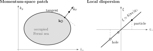
Near a regular point $\mathbf k_{\mathrm F}$, only the normal displacement $q_\perp$ changes the energy to first order. The local dispersion is $\xi\approx\hbar|\mathbf v_{\mathrm F}|q_\perp$; a hole lies just inside the occupied region and a particle lies just outside. Tangential displacement probes curvature only beyond leading order.

Free-particle sphere

For

$$\epsilon(k) = \frac{\hbar^2k^2}{2m},$$

the surface is a sphere and

$$\mu_0 = E_{\mathrm F} = \frac{\hbar^2k_{\mathrm F}^2}{2m}.$$

The Fermi velocity is

$$\mathbf v_{\mathrm F} = \frac{\hbar\mathbf k_{\mathrm F}}{m}.$$

Take a radial displacement

$$k = k_{\mathrm F} + q_r.$$

Then

$$\begin{aligned} \xi_k &= \frac{\hbar^2}{2m} \left[ (k_{\mathrm F}+q_r)^2 - k_{\mathrm F}^2 \right] \\ &= \hbar v_{\mathrm F}q_r + \frac{\hbar^2q_r^2}{2m}. \end{aligned}$$

For $|q_r|\ll k_{\mathrm F}$,

$$\xi_k \approx \hbar v_{\mathrm F}q_r.$$

Low excitation energy therefore means proximity to $k_{mathrm F}$, not proximity to $k=0$.

Particle and hole excitations

Let $|\mathrm{FS}\rangle$ denote the filled zero-temperature Fermi sea. Remove a fermion from an occupied mode $\mathbf k_h$ and place it in an unoccupied mode $\mathbf k_p$:

$$|\mathbf k_p,\mathbf k_h\rangle = c_{\mathbf k_p}^{\dagger} c_{\mathbf k_h} |\mathrm{FS}\rangle.$$

The mode conditions are

$$\xi_{\mathbf k_h}<0, \qquad \xi_{\mathbf k_p}>0.$$

For the ideal gas, the excitation energy is

$$\Delta E = \xi_{\mathbf k_p} - \xi_{\mathbf k_h},$$

and the momentum transfer is

$$\Delta\mathbf P = \hbar (\mathbf k_p-\mathbf k_h).$$

Both $\mathbf k_p$ and $\mathbf k_h$ can have magnitudes of order $k_{\mathrm F}$ while $\Delta E$ is arbitrarily small in the thermodynamic limit. The small quantity is their normal distance from the Fermi surface.

A hole is a missing occupation relative to the filled reference sea. It is not an additional microscopic species. Continuum kinematics and response require summing this elementary promotion over all allowed initial states and belong to the dedicated excitation treatment.

Why low-energy physics lives near the surface

Suppose a probe supplies an energy scale $\Delta\ll E_{\mathrm F}$. A state can change occupation only if

$$|\xi_{\mathbf k}| \lesssim \Delta.$$

Using local linearization, the corresponding normal shell thickness is

$$|q_\perp| \lesssim \frac{\Delta} {\hbar|\mathbf v_{\mathrm F}|}.$$

The shell is thin in the normal direction but extends over the full Fermi surface. Consequently, low-energy sums separate naturally into:

• an integral over Fermi-surface position;
• an integral over the small normal energy $\xi$;
• internal spin, band, or flavor sums.

This structure underlies:

• linear low-temperature heat capacity;
• Pauli spin response;
• screening and density response;
• particle–hole continua;
• Cooper pairing;
• quasiparticle scattering restrictions;
• transport dominated by selected surface regions.

The statement has limits. A gapped system, a one-dimensional Luttinger liquid, a non-Fermi liquid, or a system without translational invariance may require different low-energy variables. Low-Dimensional Quantum Gases explains the ideal Fermi-point geometry and why interactions make the one-dimensional case special.

Surface representation of the density of states

For one smooth band, the density of states per $d$-dimensional real-space measure is

$$\frac{D(E)}{\mathcal V_d} = g \int \frac{d^dk}{(2\pi)^d} \delta\!\left[ E-\epsilon(\mathbf k) \right].$$

Using the coarea formula,

$$\frac{D(E)}{\mathcal V_d} = g \int_{\epsilon(\mathbf k)=E} \frac{dS_{\mathbf k}}{(2\pi)^d} \frac{1} {|\nabla_{\mathbf k}\epsilon|}.$$

Since

$$|\nabla_{\mathbf k}\epsilon| = \hbar|\mathbf v|,$$

the Fermi-level density of states is

$$\frac{D(E_{\mathrm F})}{\mathcal V_d} = \frac{g}{\hbar} \int_{\mathcal S_{\mathrm F}} \frac{dS_{\mathbf k}}{(2\pi)^d} \frac{1} {|\mathbf v_{\mathrm F}(\mathbf k)|}.$$

Large surface area and small Fermi velocity both enhance the density of low-energy states. At a point where $\mathbf v_{\mathrm F}=0$, the regular surface formula signals a possible singularity and must be treated with care.

For a three-dimensional free gas,

$$\frac{D(E_{\mathrm F})}{V} = g \frac{4\pi k_{\mathrm F}^2}{(2\pi)^3} \frac{m}{\hbar^2k_{\mathrm F}}.$$

Thus

$$\frac{D(E_{\mathrm F})}{V} = \frac{gm k_{\mathrm F}} {2\pi^2\hbar^2}.$$

This agrees with the derivative of the integrated state count. The canonical normalization discussion is Density of States: First Encounter.

Thermal smearing

At nonzero temperature, the Fermi–Dirac occupation is smooth. With

$$\xi = \epsilon-\mu(T),$$

one has

$$f(\xi) = \frac{1} {e^{\xi/(k_{\mathrm B}T)}+1}.$$

The thermal weighting function is

$$- \frac{\partial f}{\partial\xi} = \frac{1} {4k_{\mathrm B}T} \operatorname{sech}^2\!\left( \frac{\xi}{2k_{\mathrm B}T} \right).$$

It is centered at $\xi=0$ and has width of order $k_{\mathrm B}T$. Near a regular surface point, this corresponds to

$$\delta k_T \sim \frac{k_{\mathrm B}T} {\hbar|\mathbf v_{\mathrm F}|}.$$

For an isotropic quadratic dispersion,

$$\frac{\delta k_T}{k_{\mathrm F}} \sim \frac{1}{2} \frac{T}{T_{\mathrm F}}.$$

At $T>0$, there is no literal discontinuity in $n(\mathbf k)$. Phrases such as the finite-temperature Fermi surface usually mean one of:

• the underlying zero-temperature surface;
• the locus $\epsilon(\mathbf k)=\mu(T)$ in an ideal band;
• the ridge of low-energy spectral weight;
• a surface inferred by extrapolating measured dispersions.

Those definitions agree in a simple low-temperature Fermi liquid but need not agree in a strongly broadened or pseudogapped system. The thermally active shell is developed in Degenerate Fermi Gas.

Relation to conventional metals

In an ideal periodic crystal, each Bloch band provides energies $E_n(\mathbf k)$ in the Brillouin zone. A conventional metal has at least one band that crosses the chemical potential, producing gapless particle and hole excitations near

$$E_n(\mathbf k) = \mu_0.$$

A conventional band insulator instead has completely filled bands below a gap and empty bands above it. There is no regular Fermi surface at the chemical potential.

This gives the basic contrast:

State	Chemical-potential structure	Low-energy single-particle phase space
Conventional metal	one or more bands cross $\mu_0$	Fermi-surface excitations
Band insulator	$\mu_0$ lies in a gap	no gapless charged band excitations
Semimetal	touching points, lines, or small pockets	reduced or pocket-dependent phase space

The Fermi surface does more than certify that a band is partially filled. Its local velocity, curvature, orbital content, and scattering rate control how different regions contribute to transport and spectroscopy.

Fermi Surface in Quantum Matter develops these band-specific statements, including electron and hole pockets, Brillouin-zone periodicity, topology changes, and experimental reconstruction.

Anisotropic quadratic example

Consider

$$\epsilon(\mathbf k) = \frac{\hbar^2}{2} \left( \frac{k_x^2}{m_x} + \frac{k_y^2}{m_y} + \frac{k_z^2}{m_z} \right).$$

The Fermi surface is the ellipsoid

$$\frac{k_x^2}{k_{{\mathrm F}x}^2} + \frac{k_y^2}{k_{{\mathrm F}y}^2} + \frac{k_z^2}{k_{{\mathrm F}z}^2} = 1,$$

with semiaxes

$$k_{{\mathrm F}i} = \frac{\sqrt{2m_iE_{\mathrm F}}}{\hbar}.$$

The Fermi velocity is

$$\mathbf v_{\mathrm F} = \hbar \left( \frac{k_x}{m_x}, \frac{k_y}{m_y}, \frac{k_z}{m_z} \right)_{\mathcal S_{\mathrm F}}.$$

Except along principal axes, $\mathbf v_{\mathrm F}$ is not parallel to $\mathbf k$. It remains normal to the ellipsoid because it is proportional to the gradient of the band energy.

Fermi-surface topology preview

A Fermi surface can have several disconnected components. As density, pressure, field, or another parameter changes, components can appear, disappear, join through a neck, or change from closed to open within a Brillouin-zone representation.

A zero-temperature change in Fermi-surface topology without conventional symmetry breaking is often called a Lifshitz transition. At the transition, the chemical potential crosses a critical point of the dispersion:

$$\nabla_{\mathbf k}\epsilon = 0.$$

This page uses the idea only to mark where regular-surface formulas can fail. The topology, pocket language, and associated thermodynamic signatures belong to Quantum Matter.

Interactions and the quasiparticle surface

Weak or moderate interactions do not necessarily destroy the organizing surface. In a Landau Fermi liquid, long-lived quasiparticles near the chemical potential have a renormalized dispersion $\xi_{\mathbf k}^{*}$, and the quasiparticle Fermi surface is

$$\xi_{\mathbf k}^{*} = 0.$$

Near a regular point,

$$\xi_{\mathbf k}^{*} \approx \hbar \mathbf v_{\mathrm F}^{*} \cdot (\mathbf k-\mathbf k_{\mathrm F}).$$

The retarded Green function has the schematic low-energy form

$$G^R(\mathbf k,E) \approx \frac{Z_{\mathbf k}} {E-\xi_{\mathbf k}^{*}+i\Gamma_{\mathbf k}} + G_{\mathrm{inc}}^R.$$

Here $Z_{\mathbf k}$ is the quasiparticle residue, $\Gamma_{\mathbf k}$ is a width, and $G_{\mathrm{inc}}^R$ is an incoherent contribution. At $T=0$ in a conventional Fermi liquid, the momentum distribution has a jump of height $Z$ rather than the ideal-gas jump of height one.

The surface is therefore more robust than the ideal occupation step, but this statement has boundaries:

• a superconductor gaps the normal-state Fermi surface except at possible nodes;
• a density wave can reconstruct the surface by enlarging the real-space unit cell;
• a Mott insulator can invalidate a band-filling picture;
• a one-dimensional interacting gas generally has Fermi points without Landau quasiparticles;
• a non-Fermi liquid may have sharp low-energy momentum structure without a simple pole;
• Green-function zeros can complicate generalized surface definitions.

Detailed quasiparticle dynamics and Landau parameters are developed in the dedicated Fermi-liquid treatment below.

Luttinger-volume preview

For the noninteracting continuum gas, particle density is exactly the occupied $k$-space volume divided by $(2\pi)^d$, including internal multiplicity. Luttinger’s theorem shows that a related volume constraint survives interactions for broad classes of translationally invariant fermion systems.

The careful statement depends on:

• conserved particle number;
• translational symmetry or a stated enlarged unit cell;
• how filled bands are counted;
• analyticity and adiabatic-continuity assumptions;
• whether topological order or fractionalization is present;
• whether poles, sign changes, or zeros of the Green function define the boundary.

It is therefore unsafe to summarize the theorem as “interactions never change the Fermi surface.” Interactions can change the shape, velocity, residue, and even the phase itself. Under the theorem’s assumptions, the constrained quantity is the appropriate enclosed volume modulo filled-band contributions, not every local geometric feature.

Experimental access

No single instrument displays an abstract Fermi surface without modeling. Different probes infer complementary aspects.

Angle-resolved photoemission

In a common approximation, photoemission intensity has the schematic form

$$I(\mathbf k,E) \propto |M(\mathbf k,E)|^2 f(E) A(\mathbf k,E),$$

where $A$ is the one-particle spectral function, $f$ is the occupation factor, and $M$ is a matrix element. Low-energy spectral-weight ridges can map occupied portions of a material’s Fermi surface.

Matrix elements, surface sensitivity, energy resolution, lifetime broadening, and inaccessible unoccupied states all matter. ARPES measures a spectral intensity, not an unqualified geometric contour.

Quantum oscillations

In a magnetic field, semiclassical cyclotron orbits quantize. The oscillation frequency $F$ is related to an extremal momentum-space orbit area $A_{\mathrm{ext}}$ by the Onsager relation

$$F = \frac{\hbar} {2\pi|q|} A_{\mathrm{ext}}.$$

Quantum oscillations provide precise extremal areas and effective masses in sufficiently coherent samples, but reconstructing a full three-dimensional surface requires angular scans and a band model.

Ultracold gases

Time-of-flight and momentum-resolved probes can estimate occupation distributions in atomic gases. Trapping, interactions during expansion, finite temperature, imaging resolution, and component imbalance must be included before identifying an observed edge with a homogeneous $k_{\mathrm F}$.

These methods are introduced here only to show how the concept connects to measurements. Their detailed theory belongs to Quantum Matter, AMO, and experimental-method pages.

Surface does not mean every state is active

At $T=0$, the number of particles occupies the entire Fermi sea:

$$N \propto V_{\mathrm F}^{(k)}.$$

Low-energy thermodynamics depends on a shell near the boundary:

$$\delta N_{\mathrm{active}} \sim D(E_{\mathrm F}) k_{\mathrm B}T.$$

These are different counts. The surface organizes the states that can change occupation at low energy; it does not imply that all other occupied states disappear or cease contributing to the ground-state energy and pressure.

For a three-dimensional ideal gas,

$$\frac{\delta N_{\mathrm{active}}}{N} = O\!\left( \frac{T}{T_{\mathrm F}} \right).$$

The precise coefficient depends on which thermal weighting or excitation count is meant.

Practical interpretation workflow

When a Fermi surface appears in a calculation or experiment:

1. Identify the momentum label. Decide whether it is continuum wave vector, crystal momentum, or a quasiparticle label.
2. State the reference energy. Specify $\mu_0$, the band zero, and whether rest energy is subtracted.
3. List bands and internal components. Avoid hiding spin, valley, or pocket multiplicities.
4. Locate regular crossings. Solve $E_n(\mathbf k)=\mu_0$ and test $\nabla_{\mathbf k}E_n\ne0$.
5. Compute local velocities. The gradient, not the radial direction, fixes $\mathbf v_{\mathrm F}$.
6. Separate sea volume from surface properties. Density is a volume count; low-energy response is surface weighted.
7. Check temperature and lifetime. A broad edge may not define a unique experimental contour.
8. Check interactions and broken symmetry. Decide whether a band, quasiparticle, reconstructed, paired, or non-Fermi-liquid description is intended.

Canonical boundaries

This page owns:

• the generic Fermi-sea and Fermi-surface distinction;
• the regular level-set definition in continuum many-body language;
• the Fermi velocity as the local surface normal;
• local linearization and normal-versus-tangential displacements;
• elementary particle and hole excitations near the surface;
• the surface representation of the density of states;
• thermal smearing and the meaning of a finite-temperature surface;
• the bridge from ideal gases to conventional metals and Fermi liquids;
• carefully bounded previews of Luttinger volume and experimental access.

Other pages own:

• dimension-by-dimension density, momentum, energy, and degeneracy formulas: Fermi Momentum and Fermi Energy;
• the complete uniform ideal-gas thermodynamics: Ideal Fermi Gas;
• the low-temperature active shell, heat capacity, and Pauli blocking: Degenerate Fermi Gas;
• Fermi–Dirac occupation and its thermal window: Fermi–Dirac Statistics;
• particle–hole intermediate states, small denominators, and infrared perturbative counting: Perturbation Theory in Many-Body Systems;
• the generic excitation concept, hole quantum numbers, continuum kinematics, and response support: Particle–Hole Excitations;
• resummation of the independent continuum into screened density response and collective poles: Random Phase Approximation;
• quasiparticle lifetime, effective mass, and Landau parameters: Fermi Liquid Theory Preview;
• Bloch-band topology, pockets, Lifshitz transitions, quantum oscillations, and material-specific surfaces: Fermi Surface in Quantum Matter;
• low-temperature asymptotic integration: Sommerfeld Expansion.

Common mistakes

Confusing the surface with the sea

The Fermi sea is the occupied $d$-dimensional region. The Fermi surface is its $(d-1)$-dimensional boundary when the crossing is regular.

Treating the surface as a real-space interface

It is a structure in wave-vector or crystal-momentum space. A sample boundary is a different physical object.

Assuming every Fermi surface is spherical

A sphere follows from isotropy and a monotone radial dispersion. Crystal bands and anisotropic masses generally produce nonspherical surfaces.

Assuming velocity is parallel to wave vector

The velocity is $\hbar^{-1}\nabla_{\mathbf k}\epsilon$. It is normal to a constant-energy surface and need not point along $\mathbf k$.

Defining a sharp surface at arbitrary temperature

Finite-temperature occupations are smooth. State which operational definition is being used.

Equating Fermi energy with chemical potential at every temperature

$E_{\mathrm F}$ is a zero-temperature density scale. The fixed-density chemical potential generally shifts with temperature.

Counting surface area to obtain particle number

Particle number depends on enclosed wave-vector volume. Surface area enters low-energy density-of-states and response integrals.

Assuming a Fermi surface proves Landau quasiparticles exist

One-dimensional and non-Fermi-liquid systems can retain sharp momentum-space structure without conventional quasiparticle poles.

Saying interactions cannot change the Fermi surface

Interactions can deform, reconstruct, gap, or destroy the surface. Luttinger-type volume constraints hold only under stated assumptions.

Reading a probe as a direct photograph

ARPES, quantum oscillations, and momentum imaging each contain matrix elements, resolution limits, and model-dependent reconstruction.

Exercises

Prove that the Fermi velocity is normal

Let a regular Fermi surface be defined by

$$\epsilon(\mathbf k) = \mu_0.$$

Show that the Fermi velocity is orthogonal to every tangent vector at $\mathbf k_{\mathrm F}$.

Solution

Let $\mathbf k(s)$ be any curve lying in the Fermi surface with

$$\mathbf k(0) = \mathbf k_{\mathrm F}.$$

Along the curve,

$$\epsilon[\mathbf k(s)] = \mu_0.$$

Differentiate at $s=0$:

$$0 = \left. \frac{d\epsilon}{ds} \right|_{s=0} = \nabla_{\mathbf k}\epsilon(\mathbf k_{\mathrm F}) \cdot \left. \frac{d\mathbf k}{ds} \right|_{s=0}.$$

The derivative $d\mathbf k/ds$ is an arbitrary tangent vector. Since

$$\mathbf v_{\mathrm F} = \frac{1}{\hbar} \nabla_{\mathbf k}\epsilon,$$

$\mathbf v_{\mathrm F}$ is orthogonal to every tangent vector and is therefore normal to the surface.

Linearize the free-particle dispersion

For a three-dimensional free particle, set $k=k_{\mathrm F}+q_r$. Derive the exact expression for $\xi_k$ and determine the relative size of the quadratic correction to the linear term.

Solution

Using

$$\xi_k = \frac{\hbar^2}{2m} (k^2-k_{\mathrm F}^2),$$

one obtains

$$\xi_k = \frac{\hbar^2}{2m} \left( 2k_{\mathrm F}q_r + q_r^2 \right).$$

Since $v_{\mathrm F}=\hbar k_{\mathrm F}/m$,

$$\xi_k = \hbar v_{\mathrm F}q_r + \frac{\hbar^2q_r^2}{2m}.$$

The ratio of the quadratic term to the linear term is

$$\frac{ \hbar^2q_r^2/(2m) }{ \hbar v_{\mathrm F}|q_r| } = \frac{|q_r|}{2k_{\mathrm F}}.$$

The linearization is controlled by $|q_r|/k_{\mathrm F}\ll1$.

Derive the surface density of states

Starting from

$$\frac{D(E)}{\mathcal V_d} = g \int \frac{d^dk}{(2\pi)^d} \delta[E-\epsilon(\mathbf k)],$$

introduce a local normal coordinate and derive the surface integral.

Solution

Near a regular constant-energy surface, use coordinates $(s_1,\ldots,s_{d-1},q_\perp)$, where the $s_i$ lie along the surface and $q_\perp$ is normal. To leading order,

$$d^dk = dS_{\mathbf k}\,dq_\perp,$$

and

$$E-\epsilon(\mathbf k) \approx - |\nabla_{\mathbf k}\epsilon| q_\perp.$$

Therefore

$$\delta[E-\epsilon(\mathbf k)] = \frac{ \delta(q_\perp) }{ |\nabla_{\mathbf k}\epsilon| }.$$

The normal integral gives

$$\frac{D(E)}{\mathcal V_d} = g \int_{\epsilon=E} \frac{dS_{\mathbf k}}{(2\pi)^d} \frac{1} {|\nabla_{\mathbf k}\epsilon|}.$$

Using $|\nabla_{\mathbf k}\epsilon|=\hbar|\mathbf v|$ gives the velocity form.

Check the free-gas density of states

Apply the surface formula to a three-dimensional sphere and recover

$$\frac{D(E_{\mathrm F})}{V} = \frac{gm k_{\mathrm F}} {2\pi^2\hbar^2}.$$

Then show that it equals $3n/(2E_{\mathrm F})$.

Solution

The Fermi-sphere area is $4\pi k_{\mathrm F}^2$, and

$$|\nabla_{\mathbf k}\epsilon| = \frac{\hbar^2k_{\mathrm F}}{m}.$$

Thus

$$\begin{aligned} \frac{D(E_{\mathrm F})}{V} &= g \frac{4\pi k_{\mathrm F}^2}{(2\pi)^3} \frac{m}{\hbar^2k_{\mathrm F}} \\ &= \frac{gm k_{\mathrm F}} {2\pi^2\hbar^2}. \end{aligned}$$

Using

$$n = \frac{gk_{\mathrm F}^3}{6\pi^2}$$

and

$$E_{\mathrm F} = \frac{\hbar^2k_{\mathrm F}^2}{2m},$$

one finds

$$\frac{3n}{2E_{\mathrm F}} = \frac{gm k_{\mathrm F}} {2\pi^2\hbar^2}.$$

Estimate the thermal shell

Use local linearization to derive the thermally broadened momentum scale. Specialize to an isotropic quadratic dispersion and express the result as a fraction of $k_{\mathrm F}$.

Solution

Thermal changes in occupation occur over

$$|\xi| \sim k_{\mathrm B}T.$$

Since

$$\xi \approx \hbar|\mathbf v_{\mathrm F}|q_\perp,$$

the normal width is

$$\delta k_T \sim \frac{k_{\mathrm B}T} {\hbar|\mathbf v_{\mathrm F}|}.$$

For a quadratic dispersion,

$$v_{\mathrm F} = \frac{\hbar k_{\mathrm F}}{m}.$$

Therefore

$$\frac{\delta k_T}{k_{\mathrm F}} \sim \frac{mk_{\mathrm B}T} {\hbar^2k_{\mathrm F}^2} = \frac{k_{\mathrm B}T} {2E_{\mathrm F}} = \frac{T}{2T_{\mathrm F}}.$$

Analyze an anisotropic ellipsoid

For the anisotropic quadratic dispersion on this page, derive the occupied $k$-space volume and the density as a function of $E_{\mathrm F}$.

Solution

The ellipsoid semiaxes are

$$k_{{\mathrm F}i} = \frac{\sqrt{2m_iE_{\mathrm F}}}{\hbar}.$$

Its volume is

$$V_{\mathrm F}^{(k)} = \frac{4\pi}{3} k_{{\mathrm F}x} k_{{\mathrm F}y} k_{{\mathrm F}z}.$$

Substitution gives

$$V_{\mathrm F}^{(k)} = \frac{4\pi}{3} \left( \frac{2E_{\mathrm F}}{\hbar^2} \right)^{3/2} (m_xm_ym_z)^{1/2}.$$

Including internal degeneracy,

$$n = g \frac{V_{\mathrm F}^{(k)}}{(2\pi)^3}.$$

Therefore

$$n = \frac{g}{6\pi^2} \left( \frac{2E_{\mathrm F}}{\hbar^2} \right)^{3/2} (m_xm_ym_z)^{1/2}.$$

The geometric-mean mass $(m_xm_ym_z)^{1/3}$ controls the enclosed-volume relation, while directional velocities retain the individual masses.

Compute a particle–hole excitation

For a free isotropic gas, take

$$\mathbf k_h = (k_{\mathrm F}-q_h) \widehat{\mathbf n}_h,$$

and

$$\mathbf k_p = (k_{\mathrm F}+q_p) \widehat{\mathbf n}_p,$$

where $q_h,q_p\ll k_{\mathrm F}$. Find the leading excitation energy and momentum transfer.

Solution

Linearization gives

$$\xi_{\mathbf k_p} \approx \hbar v_{\mathrm F}q_p,$$

and

$$\xi_{\mathbf k_h} \approx - \hbar v_{\mathrm F}q_h.$$

Hence

$$\Delta E = \xi_{\mathbf k_p} - \xi_{\mathbf k_h} \approx \hbar v_{\mathrm F} (q_p+q_h).$$

The momentum transfer is

$$\Delta\mathbf P = \hbar \left[ (k_{\mathrm F}+q_p) \widehat{\mathbf n}_p - (k_{\mathrm F}-q_h) \widehat{\mathbf n}_h \right].$$

The excitation energy can be arbitrarily small as $q_p,q_h\to0$, even when the momentum transfer remains of order $\hbar k_{\mathrm F}$ because the two surface normals differ substantially.

Compare a metal and a filled band

Explain why a partially filled regular band has arbitrarily low-energy particle–hole excitations in the thermodynamic limit, while an isolated completely filled band does not.

Solution

In a partially filled regular band, there are occupied states with energies arbitrarily close below $\mu_0$ and empty states arbitrarily close above it. In the thermodynamic limit, the allowed $\mathbf k$ values become dense, so a particle can be moved across the Fermi surface with

$$\Delta E \longrightarrow 0.$$

For an isolated completely filled band, every state in that band is occupied. The nearest empty one-particle states lie in another band separated by a gap $E_g$. A charged particle–hole excitation across the gap therefore costs at least an energy approaching $E_g$, apart from interaction-induced bound-state corrections.

The argument distinguishes a conventional band metal from a band insulator. It does not by itself classify Mott insulators, superconductors, or topologically ordered phases.

Cross-links

• Fermi Momentum and Fermi Energy
• Ideal Fermi Gas
• Degenerate Fermi Gas
• Fermi–Dirac Statistics
• Occupation Numbers
• Chemical Potential
• Thermodynamic Limit
• Density of States: First Encounter
• Spectral Representation
• Pauli Exclusion Principle
• Ideal Fermi Gas Model Card

References

• N. W. Ashcroft and N. D. Mermin, Solid State Physics, Holt, Rinehart and Winston (1976) — free-electron surfaces, band crossings, and transport geometry.
• A. A. Abrikosov, L. P. Gorkov, and I. E. Dzyaloshinski, Methods of Quantum Field Theory in Statistical Physics, Dover (1975) — Green functions and interacting Fermi systems.
• D. Pines and P. Nozières, The Theory of Quantum Liquids, Vol. I: Normal Fermi Liquids, W. A. Benjamin (1966) — quasiparticles and Fermi-liquid response.
• G. Baym and C. Pethick, Landau Fermi-Liquid Theory, Wiley (1991) — low-energy quasiparticles and Fermi-surface deformations.
• G. F. Giuliani and G. Vignale, Quantum Theory of the Electron Liquid, Cambridge University Press (2005) — electron-liquid response and Fermi-surface conventions.
• J. M. Luttinger, “Fermi surface and some simple equilibrium properties of a system of interacting fermions,” Physical Review 119, 1153–1163 (1960) — interacting Fermi-volume relation and its assumptions.
• A. Damascelli, Z. Hussain, and Z.-X. Shen, “Angle-resolved photoemission studies of the cuprate superconductors,” Reviews of Modern Physics 75, 473–541 (2003) — spectral-function interpretation and experimental Fermi-surface mapping.
• J. A. Sobota, Y. He, and Z.-X. Shen, “Angle-resolved photoemission studies of quantum materials,” Reviews of Modern Physics 93, 025006 (2021) — modern ARPES methods and limitations.
• S. Giorgini, L. P. Pitaevskii, and S. Stringari, “Theory of ultracold atomic Fermi gases,” Reviews of Modern Physics 80, 1215–1274 (2008) — Fermi surfaces and momentum distributions in atomic gases.