Fermi–Dirac Statistics

Fermi–Dirac statistics gives the equilibrium occupation of ideal fermionic modes. For a mode $i$ with one-particle energy $\epsilon_i$,

$$\overline n_i = \frac{1}{ e^{\beta(\epsilon_i-\mu)}+1 }, \qquad \beta = \frac{1}{k_{\mathrm B}T}.$$

The plus sign in the denominator follows from the fermionic occupation rule

$$n_i \in \{0,1\}.$$

Every complete one-particle mode is either empty or occupied by one fermion. The mean $\overline n_i$ can lie anywhere between zero and one because it is an ensemble average, not a fractional eigenvalue.

This page owns the derivation, interpretation, fluctuations, and limiting behavior of the Fermi–Dirac occupation law. The formula card is the compact lookup entry; antisymmetry and exclusion themselves belong to Fermions and the Pauli Exclusion Principle.

Assumptions

The standard mode formula assumes:

• thermal equilibrium at temperature $T$;
• a grand-canonical description with chemical potential $\mu$;
• independent fermionic modes, or controlled quasiparticle modes with a diagonal quadratic Hamiltonian;
• well-defined one-mode energies $\epsilon_i$;
• occupations restricted to $n_i=0$ or $1$;
• a conserved particle number or charge to which $\mu$ couples.

For ideal modes,

$$H = \sum_i \epsilon_i n_i, \qquad N = \sum_i n_i.$$

The formula is exact for a noninteracting grand-canonical Fermi gas. It can also describe weakly interacting quasiparticles when an effective independent-mode picture is justified, but it is not automatically the occupation of bare microscopic modes in an interacting system.

From Antisymmetry to Thermal Occupation

Antisymmetry implies that two identical fermions cannot occupy the same complete one-particle state. In occupation language,

$$n_i^2 = n_i,$$

because the only eigenvalues are zero and one.

This kinematic restriction does not by itself produce a thermal distribution. Fermi–Dirac statistics combines:

$$\begin{gathered} \text{fermionic occupations} \\ +\ \text{equilibrium weights} \\ +\ \text{an ensemble constraint}. \end{gathered}$$

A Slater determinant, a superposition of determinants, and a thermal state all obey fermionic antisymmetry. Only the equilibrium mixed state has the Fermi–Dirac occupation probabilities derived below.

Grand-Canonical Derivation

For the grand Hamiltonian

$$K = H-\mu N,$$

independent modes give

$$K = \sum_i (\epsilon_i-\mu)n_i.$$

The grand partition function factorizes:

$$\Xi = \prod_i \xi_i.$$

One fermionic mode has only two allowed occupations, so

$$\begin{aligned} \xi_i &= \sum_{n_i=0}^{1} e^{-\beta(\epsilon_i-\mu)n_i} \\ &= 1+q_i, \end{aligned}$$

where

$$q_i \equiv e^{-\beta(\epsilon_i-\mu)}.$$

The mean occupation is

$$\begin{aligned} \overline n_i &= q_i \frac{\partial}{\partial q_i} \ln\xi_i \\ &= \frac{q_i}{1+q_i} \\ &= \frac{1}{ e^{\beta(\epsilon_i-\mu)}+1 }. \end{aligned}$$

Unlike a bosonic geometric sum, the one-mode fermionic sum is finite. For a finite set of fermionic modes, no convergence bound analogous to $\mu<\epsilon_0$ is needed for finite real $\mu$.

Infinite-mode products and continuum limits still require thermodynamic regularization and a controlled density of states. The absence of a one-mode divergence does not make every infinite-volume trace finite.

The ideal-mode grand potential is

$$\Omega_{\mathrm G} = -k_{\mathrm B}T \sum_i \ln \left[ 1+e^{-\beta(\epsilon_i-\mu)} \right].$$

The Full One-Mode Distribution

One ideal fermionic mode has a Bernoulli distribution:

$$P_i(0) = \frac{1}{1+q_i}, \qquad P_i(1) = \frac{q_i}{1+q_i}.$$

Therefore

$$P_i(1) = \overline n_i, \qquad P_i(0) = 1-\overline n_i.$$

The probability ratio is

$$\frac{P_i(1)}{P_i(0)} = q_i = e^{-\beta(\epsilon_i-\mu)}.$$

At $\epsilon_i=\mu$, the empty and occupied states have equal grand energy, so

$$P_i(0) = P_i(1) = \frac{1}{2}$$

for every finite positive temperature.

Dimensionless Profile

Define

$$x \equiv \beta(\epsilon-\mu).$$

The Fermi function is

$$f_{\mathrm F}(x) = \frac{1}{e^x+1}.$$

It is monotone, bounded, and centered at

$$f_{\mathrm F}(0) = \frac{1}{2}.$$

At low temperature it approaches a sharp step in energy. Finite temperature rounds that step over an energy interval of order $k_{\mathrm B}T$.

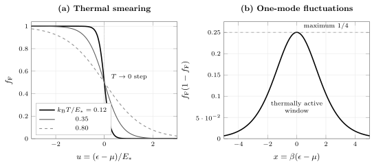
Cooling sharpens the Fermi–Dirac occupation toward a step at $\epsilon=\mu$. The one-mode variance $f_{\mathrm F}(1-f_{\mathrm F})$ is concentrated in the same thermal window and reaches its maximum $1/4$ at the chemical potential.

Pauli Blocking

For one complete fermionic mode,

$$0 \leq \overline n_i \leq 1.$$

The factor that measures availability of the mode is

$$1-\overline n_i.$$

In kinetic equations, scattering into a fermionic final state commonly carries a Pauli-blocking factor $1-f$. A fully occupied final mode cannot accept another identical fermion.

This is not a new repulsive force. The restriction comes from the antisymmetric state space and fermionic operator algebra. It changes the allowed many-particle configurations and therefore has major energetic and thermodynamic consequences.

A Mode Includes Every Quantum Label

Exclusion applies to a complete one-particle mode. For electrons, a mode may be labeled by

$$i = (\mathbf k,\sigma,b),$$

where $\mathbf k$ is momentum or crystal momentum, $\sigma$ is spin, and $b$ is a band or orbital label.

Two electrons with opposite spin can occupy the same spatial orbital because they occupy distinct spin-orbitals. If a spatial orbital has two independent spin modes with the same energy, its mean total occupation is

$$\overline N_{\mathrm{orb}} = 2f_{\mathrm F} \left[ \beta(\epsilon-\mu) \right].$$

Saying that a fermionic mode holds at most one particle does not mean that every spatial orbital, momentum value, or energy level has total capacity one.

Particle–Hole Symmetry of the Function

The dimensionless Fermi function obeys

$$f_{\mathrm F}(-x) = 1-f_{\mathrm F}(x).$$

Equivalently,

$$f_{\mathrm F}(x) + f_{\mathrm F}(-x) = 1.$$

An energy $\mu+\Delta$ above the chemical potential has the same particle occupation as the hole probability at $\mu-\Delta$ below it:

$$f_{\mathrm F} \left( \frac{\Delta}{k_{\mathrm B}T} \right) = 1- f_{\mathrm F} \left( -\frac{\Delta}{k_{\mathrm B}T} \right).$$

This identity belongs to the ideal Fermi function. A physical system need not possess an exact particle–hole symmetry in its density of states, dispersion, or interactions.

Number Fluctuations

Because $n_i^2=n_i$,

$$\langle n_i^2\rangle = \overline n_i.$$

The variance is therefore

$$\operatorname{Var}(n_i) = \overline n_i \left( 1-\overline n_i \right).$$

This is smaller than the Poisson benchmark $\operatorname{Var}(n)=\overline n$ whenever $0<\overline n<1$. Fermionic exclusion suppresses occupation fluctuations.

The variance is largest at half occupation:

$$\operatorname{Var}(n_i)_{\max} = \frac{1}{4}, \qquad \epsilon_i = \mu.$$

Modes far below $\mu$ are almost certainly occupied, and modes far above $\mu$ are almost certainly empty. Both have small variance.

Fluctuation–Response Identity

Differentiating with respect to chemical potential gives

$$\left( \frac{\partial\overline n_i}{\partial\mu} \right)_T = \beta \overline n_i \left( 1-\overline n_i \right).$$

Hence

$$\left( \frac{\partial\overline n_i}{\partial\mu} \right)_T = \beta \operatorname{Var}(n_i).$$

For independent modes,

$$\operatorname{Var}(N) = \sum_i \overline n_i \left( 1-\overline n_i \right),$$

and

$$\left( \frac{\partial\overline N}{\partial\mu} \right)_T = \beta \operatorname{Var}(N).$$

Fixed-$N$ canonical states do not have these independent grand-canonical mode fluctuations; the exact number constraint introduces correlations among occupations.

The Thermal Window

The energy derivative is

$$- \frac{\partial f_{\mathrm F}}{\partial\epsilon} = \frac{\beta}{ 4\cosh^2 \left[ \beta(\epsilon-\mu)/2 \right] }.$$

This nonnegative kernel is centered at $\epsilon=\mu$ and has unit area:

$$\int_{-\infty}^{\infty} d\epsilon \left( -\frac{\partial f_{\mathrm F}}{ \partial\epsilon} \right) = 1.$$

Its maximum is

$$\left. -\frac{\partial f_{\mathrm F}}{ \partial\epsilon} \right|_{\epsilon=\mu} = \frac{1}{4k_{\mathrm B}T}.$$

The full width at half maximum is

$$\Delta\epsilon_{\mathrm{FWHM}} = 4k_{\mathrm B}T \operatorname{arcosh}\sqrt{2} \simeq 3.53k_{\mathrm B}T.$$

Thus only states within a few $k_{\mathrm B}T$ of the chemical potential change occupation appreciably at low temperature. This fact underlies low-temperature Fermi-gas thermodynamics and the Sommerfeld expansion.

Zero-Temperature Limit

For fixed $\mu$ and $\epsilon\neq\mu$,

$$\lim_{T\to0^+} f_{\mathrm F} \left[ \beta(\epsilon-\mu) \right] = \begin{cases} 1, & \epsilon<\mu, \\ 0, & \epsilon>\mu. \end{cases}$$

Equivalently,

$$f_{\mathrm F}(\epsilon) \longrightarrow \Theta(\mu-\epsilon),$$

away from the discontinuity.

The value assigned to the ideal step at $\epsilon=\mu$ is conventional. The finite-temperature Fermi function has

$$f_{\mathrm F}(\mu) = \frac{1}{2}.$$

At zero temperature, ideal fermions fill the lowest available complete one-particle modes. The occupied region in momentum space is called the Fermi sea, and its boundary in a translationally invariant system is the Fermi surface.

Chemical Potential and Fermi Energy

For an ideal fixed-density Fermi gas at zero temperature, the chemical potential approaches the Fermi energy:

$$\mu(T=0) = \epsilon_{\mathrm F}.$$

At finite temperature, $\mu$ generally shifts with $T$ when particle number is held fixed. It need not equal the zero-temperature Fermi energy.

The dimension-by-dimension density conventions and formulas for $k_{\mathrm F}$ and $E_{\mathrm F}$ are collected in Fermi Momentum and Fermi Energy.

The distinction is even more important outside a simple ideal gas:

• in a finite system, addition and removal energies can bracket a range of chemical potentials;
• in an insulator, $\mu$ can lie in a spectral gap with no one-particle state at that energy;
• in an interacting system, $\mu$ is a many-body thermodynamic derivative;
• in nonequilibrium transport, different reservoirs can impose different chemical potentials.

The Fermi–Dirac formula uses $\epsilon_i-\mu$. It does not make $\mu$ the energy of a particular occupied particle.

Dilute Maxwell–Boltzmann Limit

When

$$x = \beta(\epsilon-\mu) \gg 1,$$

set $y=e^{-x}\ll1$. Then

$$\begin{aligned} f_{\mathrm F}(x) &= \frac{y}{1+y} \\ &= y-y^2+y^3-\cdots. \end{aligned}$$

Therefore

$$f_{\mathrm F}(x) \simeq e^{-x}.$$

The leading correction is negative:

$$f_{\mathrm F}(x) - e^{-x} = -e^{-2x} + O(e^{-3x}).$$

Fermionic exclusion reduces occupation relative to the dilute classical result. Bose and Fermi occupations both approach Maxwell–Boltzmann statistics when all relevant mode occupations are small. Classical Limit of Quantum Statistics develops the phase-space-density criterion and the leading equation-of-state correction.

Degenerate Levels

If an energy level $\epsilon$ contains $g_\epsilon$ independent fermionic modes, then

$$\overline N_\epsilon = g_\epsilon f_{\mathrm F} \left[ \beta(\epsilon-\mu) \right].$$

The maximum total occupation is $g_\epsilon$, not one.

If the modes fluctuate independently in the grand-canonical ensemble,

$$\operatorname{Var}(N_\epsilon) = g_\epsilon \overline n_\epsilon \left( 1-\overline n_\epsilon \right).$$

In a continuum approximation,

$$\overline N = \int d\epsilon\, g(\epsilon) \frac{1}{ e^{\beta(\epsilon-\mu)}+1 },$$

where $g(\epsilon)$ is the one-particle density of states including the chosen internal degeneracies.

Entropy Per Mode

The entropy of one fermionic thermal mode is the binary entropy

$$\frac{s_{\mathrm F}}{k_{\mathrm B}} = -\overline n \ln\overline n - \left( 1-\overline n \right) \ln \left( 1-\overline n \right).$$

It vanishes as $\overline n\to0$ or $\overline n\to1$ because the occupation becomes certain. It is maximal at half occupation:

$$s_{\mathrm F,max} = k_{\mathrm B}\ln2.$$

At low temperature, entropy is concentrated in modes near the chemical potential, where neither empty nor occupied is overwhelmingly certain.

Example: Electrons in Independent Orbitals

For noninteracting electrons with spin label $\sigma$,

$$H = \sum_{i,\sigma} \epsilon_i c_{i\sigma}^\dagger c_{i\sigma}.$$

Each spin-orbital has mean occupation

$$\overline n_{i\sigma} = \frac{1}{ e^{\beta(\epsilon_i-\mu)}+1 }.$$

If the two spin states are degenerate and independent,

$$\overline N_i = 2\overline n_{i\sigma}.$$

At low temperature, orbitals well below $\mu$ are nearly doubly occupied, those well above are nearly empty, and only a thermal window near $\mu$ has appreciably fractional mean occupation.

Example: One Equilibrium Quantum-Dot Level

Consider one spinless level of energy $\epsilon_d$ weakly coupled to a single equilibrium fermionic reservoir. If the empty and occupied dot states equilibrate grand canonically, then

$$P(1) = f_{\mathrm F} \left[ \beta(\epsilon_d-\mu) \right],$$

and

$$P(0) = 1-P(1).$$

At resonance, $\epsilon_d=\mu$, the level is half occupied. With several reservoirs at different chemical potentials, there is generally no single equilibrium Fermi function for the dot; rates, coupling asymmetry, and transport dynamics matter.

Example: Nucleons

Protons and neutrons are fermions. In an idealized thermal description, each species has its own occupation function and chemical potential:

$$\begin{aligned} f_p(\epsilon) &= \frac{1}{e^{\beta(\epsilon-\mu_p)}+1}, \\ f_n(\epsilon) &= \frac{1}{e^{\beta(\epsilon-\mu_n)}+1}. \end{aligned}$$

Nuclear interactions are strong, so the ideal gas is only a baseline. Nevertheless, exclusion, filled low-energy states, and thermal smearing remain organizing ideas in more realistic many-body treatments.

Example: Cold Fermionic Atoms

Ultracold fermionic atoms realize conserved fermion species with tunable density and interactions. For a noninteracting trapped or homogeneous gas, the mean occupation of each one-particle trap or momentum mode is Fermi–Dirac.

Multiple hyperfine states act as distinct internal species. Two atoms in different internal states may share the same spatial mode because their complete one-particle labels differ.

At low temperature, Pauli blocking suppresses available final states for scattering. The Degenerate Fermi Gas page connects that mode-level factor to the thin active shell, pressure, heat capacity, and cold-atom applications. Interactions, trapping, dimensionality, and pairing can move the system beyond the ideal independent-mode formula.

Finite Systems and Fixed Particle Number

In a finite grand-canonical system, $\overline N$ need not be an integer even though every number measurement yields an integer. The chemical potential is adjusted to obtain the desired mean.

For a strictly fixed-$N$ canonical system, the occupations satisfy

$$\sum_i n_i = N$$

in every microstate. One mode becoming occupied forces the allowed occupations of other modes to adjust. The factorized Bernoulli distribution is therefore not exact at finite fixed $N$.

Canonical and grand-canonical predictions often agree for local observables in a suitable thermodynamic limit, but finite-size shell structure, charging energies, exact parity, and small particle number can make their differences observable.

Interactions and Quasiparticles

In an interacting fermion system, bare mode occupations generally do not factorize. The microscopic Hamiltonian is not simply

$$H = \sum_i \epsilon_i n_i.$$

If a controlled effective theory has fermionic quasiparticles,

$$H_{\mathrm{eff}} = E_0 + \sum_\alpha E_\alpha \gamma_\alpha^\dagger\gamma_\alpha,$$

their equilibrium occupations may take the form

$$\overline n_\alpha = \frac{1}{ e^{\beta(E_\alpha-\mu_\alpha)}+1 }.$$

The effective energy, conserved charge, and chemical potential must be identified. In superconducting mean-field theory, for example, quasiparticle number is not the microscopic electron number and the excitation energies already contain the electron chemical potential.

Strong correlations can invalidate a simple quasiparticle picture. Then spectral functions and many-body correlation functions, rather than a bare Fermi function alone, determine measurable occupations and response.

Canonical Boundaries

This page owns:

• the grand-canonical derivation of the Fermi–Dirac occupation factor;
• the Bernoulli one-mode probability distribution;
• Pauli blocking in occupation language;
• mode variance and fluctuation–response relations;
• the zero-temperature step and finite-temperature smearing;
• mode-level examples for electrons, quantum dots, nucleons, and cold atoms.

Other pages own:

• antisymmetry and the exclusion principle: Composite Systems and Entanglement;
• the general Fock-space trace and number-sector statistics: Grand-Canonical Ensemble;
• the shared dilute criterion and exchange-cycle expansion: Classical Limit of Quantum Statistics;
• derivative, finite-system, and sign-convention meanings of chemical potential: Chemical Potential;
• the compact expression for quick lookup: Reference;
• the exact uniform model and state counting: Ideal Fermi Gas;
• the low-temperature regime, Pauli-blocked kinetics, pressure, heat capacity, and applications: Degenerate Fermi Gas;
• the low-temperature asymptotic method: Sommerfeld Expansion;
• generic Fermi-surface geometry and low-energy kinematics: Fermi Surface;
• electronic bands and material-specific surface topology: Quantum Matter;
• reservoir-induced currents and nonequilibrium occupations: Measurement and Open Quantum Systems.

Common Mistakes

• Treating Fermi–Dirac statistics as a consequence of exclusion alone, without equilibrium assumptions.
• Interpreting $0<\overline n_i<1$ as a fractional fermion in one measurement.
• Saying that an entire spatial orbital can hold only one electron while ignoring spin.
• Applying exclusion to an incomplete set of one-particle quantum labels.
• Calling Pauli blocking a new repulsive force.
• Assuming $\mu$ always equals the zero-temperature Fermi energy.
• Treating $f_{\mathrm F}(\mu)=1/2$ as a statement that a fixed-$N$ ground state contains half a particle in one mode.
• Forgetting that only a window of order $k_{\mathrm B}T$ is thermally active at low temperature.
• Using the Maxwell–Boltzmann approximation for deeply degenerate fermions.
• Applying independent Bernoulli mode fluctuations to a finite fixed-$N$ state.
• Counting a degeneracy factor twice when integrating over a density of states.
• Applying the bare ideal-gas formula unchanged to a strongly interacting or paired system.
• Using one equilibrium Fermi function for a device attached to reservoirs with different $(T,\mu)$.

Exercises

Derive the Bernoulli distribution

For one fermionic mode, let

$$q = e^{-\beta(\epsilon-\mu)}.$$

Derive $P(0)$, $P(1)$, and $\overline n$.

Solution

The allowed occupations are zero and one, so

$$\xi = 1+q.$$

The normalized probabilities are

$$P(0) = \frac{1}{1+q}, \qquad P(1) = \frac{q}{1+q}.$$

Therefore

$$\begin{aligned} \overline n &= 0P(0)+1P(1) \\ &= \frac{q}{1+q} \\ &= \frac{1}{e^{\beta(\epsilon-\mu)}+1}. \end{aligned}$$

Prove the particle–hole identity

Show that

$$f_{\mathrm F}(-x) = 1-f_{\mathrm F}(x).$$

Solution

Starting from the left side,

$$\begin{aligned} f_{\mathrm F}(-x) &= \frac{1}{e^{-x}+1} \\ &= \frac{e^x}{1+e^x}. \end{aligned}$$

Meanwhile,

$$\begin{aligned} 1-f_{\mathrm F}(x) &= 1- \frac{1}{e^x+1} \\ &= \frac{e^x}{1+e^x}. \end{aligned}$$

The expressions are equal. This functional identity does not require the physical density of states to be particle–hole symmetric.

Two spin modes in one orbital

A spatial orbital has two independent spin modes with the same energy. Let each have occupation probability $f$. Find the probabilities for total orbital occupation $N=0,1,2$, its mean, and its variance.

Solution

The two spin occupations are independent Bernoulli variables. Therefore

$$\begin{aligned} P(N=0) &= (1-f)^2, \\ P(N=1) &= 2f(1-f), \\ P(N=2) &= f^2. \end{aligned}$$

The mean is

$$\overline N = 2f,$$

and independence gives

$$\operatorname{Var}(N) = 2f(1-f).$$

The orbital can contain two electrons because the spin-up and spin-down states are distinct complete one-particle modes.

Find the thermal-window width

The derivative kernel is

$$- \frac{\partial f_{\mathrm F}}{\partial\epsilon} = \frac{1}{4k_{\mathrm B}T} \operatorname{sech}^2 \left( \frac{\epsilon-\mu}{2k_{\mathrm B}T} \right).$$

Find its full width at half maximum.

Solution

Half maximum requires

$$\operatorname{sech}^2 y = \frac{1}{2},$$

so

$$\cosh y = \sqrt2, \qquad |y| = \operatorname{arcosh}\sqrt2.$$

Since

$$y = \frac{\epsilon-\mu}{2k_{\mathrm B}T},$$

the two half-maximum points are separated by

$$\begin{aligned} \Delta\epsilon_{\mathrm{FWHM}} &= 4k_{\mathrm B}T \operatorname{arcosh}\sqrt2 \\ &\simeq 3.53k_{\mathrm B}T. \end{aligned}$$

Derive total number response

For independent fermionic modes, show that

$$\left( \frac{\partial\overline N}{\partial\mu} \right)_T = \beta \operatorname{Var}(N).$$

Solution

For each mode,

$$\frac{\partial\overline n_i}{\partial\mu} = \beta \overline n_i \left( 1-\overline n_i \right).$$

Summing gives

$$\frac{\partial\overline N}{\partial\mu} = \beta \sum_i \overline n_i \left( 1-\overline n_i \right).$$

Independent occupations have additive variances:

$$\begin{aligned} \operatorname{Var}(N) &= \sum_i \operatorname{Var}(n_i) \\ &= \sum_i \overline n_i \left( 1-\overline n_i \right). \end{aligned}$$

Combining the two results proves the identity.

Cross-Links

• Fermi Gas Formula Sheet
• Quantum Statistics Overview
• Maxwell–Boltzmann Limit
• Grand-Canonical Ensemble
• Fermi–Dirac Distribution Formula Card
• Ideal Fermi Gas
• Fermi Momentum and Fermi Energy
• Fermi Surface
• Bose–Einstein Statistics
• Fermions
• Pauli Exclusion Principle
• Fermionic Fock Space
• Fermionic Anticommutation Relations
• Number Operators
• Mesoscopic Transport
• Thermodynamic Limit

References

• R. K. Pathria and P. D. Beale, Statistical Mechanics, 3rd ed., Elsevier (2011).
• K. Huang, Statistical Mechanics, 2nd ed., Wiley (1987).
• M. Kardar, Statistical Physics of Particles, Cambridge University Press (2007).
• L. D. Landau and E. M. Lifshitz, Statistical Physics, Part 1, 3rd ed., Butterworth–Heinemann (1980).
• A. L. Fetter and J. D. Walecka, Quantum Theory of Many-Particle Systems, Dover (2003).
• N. W. Ashcroft and N. D. Mermin, Solid State Physics, Holt, Rinehart and Winston (1976).
• G. D. Mahan, Many-Particle Physics, 3rd ed., Springer (2000).
• S. Giorgini, L. P. Pitaevskii, and S. Stringari, “Theory of ultracold atomic Fermi gases,” Reviews of Modern Physics 80, 1215–1274 (2008).