Wave Mechanics Foundations

Wave mechanics is the coordinate-space realization of the abstract quantum formalism. A state becomes a wavefunction only after a representation is chosen; the Hamiltonian and its domain determine the evolution; and the Born density, current, boundary conditions, and normalization together determine how probability is interpreted and conserved.

This chapter supplies the technical foundation needed before solving wells, barriers, oscillators, central potentials, or time-dependent wave-packet problems. It deliberately stops before those model-specific calculations.

Helpful background. State Vectors supplies the abstract state and basis language. Born Rule for Continuous Outcomes supplies the probability measure represented by a coordinate-space amplitude.

From states to conservation laws

The central translation is

$$|\psi(t)\rangle \longrightarrow \psi(\mathbf r,t)=\langle\mathbf r|\psi(t)\rangle \longrightarrow i\hbar\,\partial_t\psi=\hat H\psi.$$

For one spinless particle of mass $m$ in a real scalar potential,

$$\hat H = -\frac{\hbar^2}{2m}\nabla^2+V(\mathbf r,t),$$

provided that the coordinate domain and the operator domain are also stated. The same differential expression can describe a particle on the line, in an interval, on a ring, or on a half-line. Those are different quantum problems because their Hilbert spaces or boundary conditions differ.

The resulting probability density and current are

$$\rho=|\psi|^2, \qquad \mathbf j = \frac{\hbar}{m}\operatorname{Im}(\psi^*\nabla\psi),$$

and, under the stated scalar-potential assumptions, they obey

$$\partial_t\rho+\nabla\cdot\mathbf j=0.$$

This local equation, its integral form, and the boundary form of the Hamiltonian are complementary tests of probability-preserving dynamics.

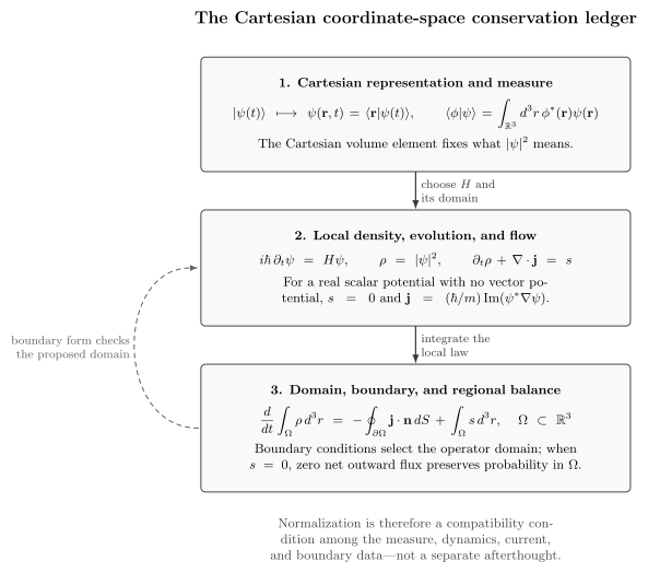
The Cartesian coordinate-space ledger. Representation supplies $\psi$; dynamics determines $\rho$ and $\mathbf j$; the domain and boundary flux determine whether the modeled region preserves total probability.

The nine-page foundation

Read	Canonical page	Capability gained
1	Coordinate Representation	Translate kets, inner products, and operators into coordinate amplitudes and kernels.
2	Wavefunctions and Probability Density	Interpret $\lvert\psi\rvert^2$ relative to the correct measure, including internal and many-particle labels.
3	Time-Dependent Schrödinger Equation in Coordinate Space	Pose a well-defined initial-value problem and distinguish the differential expression from its domain.
4	Time-Independent Schrödinger Equation	Formulate stationary spectral and boundary-value problems without treating every state as stationary.
5	Hamiltonians in Coordinate Space	Build kinetic, potential, effective, and electromagnetic differential operators with stated assumptions.
6	Probability Current	Compute direction and magnitude of probability flow, including scattering flux and gauge coupling.
7	Continuity Equation	Derive local and integral conservation and identify legitimate source or sink terms.
8	Boundary Conditions	Derive endpoint and interface conditions and connect them to self-adjointness and flux.
9	Normalization Conventions	Move correctly among square, box, delta, energy, flux, radial, and numerical normalization.

The order is conceptual rather than a demand to read every page linearly. A reader checking a scattering calculation may go directly from current to normalization; a reader setting up an eigenvalue problem may go from the TISE to boundary conditions. The prerequisite notes on each page say which earlier capabilities are actually used.

A complete problem specification

Before solving a coordinate-space problem, record the following data:

1. the configuration space and integration measure;
2. the state components, including spin or channel labels;
3. the Hamiltonian differential expression and its regime of validity;
4. the operator domain, endpoint, interface, or asymptotic conditions;
5. the initial state for a time-evolution problem, or the spectral parameter and admissibility conditions for a stationary problem;
6. the normalization convention and the observable being computed;
7. a conservation, dimensional, limiting-case, or residual check.

Writing only

$$-\frac{\hbar^2}{2m}\psi''+V\psi=E\psi$$

does not yet specify a spectrum. Likewise, writing a normalized array does not show that it represents the continuum norm or lies in the domain of the Hamiltonian.

Conservation and domain checks

For a fixed region $\Omega$, the continuity equation gives

$$\frac{d}{dt}\int_\Omega\rho\,d^3r = -\int_{\partial\Omega}\mathbf j\cdot d\mathbf S.$$

This identity separates three cases that are often conflated:

• a closed system on all space, where the asymptotic flux vanishes;
• a finite closed domain, where the boundary condition makes the net outward flux vanish;
• an open or effective description, where probability may cross the selected boundary or a controlled source term may represent gain or loss.

A decreasing norm is therefore not automatically a numerical error, and a constant norm is not by itself proof that the spatial discretization has the correct Hamiltonian domain. The model and the check must be stated together.

Quick lookup without duplicated derivations

The Probability Current formula card and Continuity Equation formula card collect the formulas, symbols, assumptions, and calculation checks. Their canonical articles in this chapter retain the derivations, interpretation, examples, limitations, and exercises.

Continue to model calculations

Use these foundations in the neighboring treatments of free particles, wells, barriers, oscillators, and central potentials. Scaling, stationary-state expansions, and qualitative bound-state theorems supply further tools for comparing and checking models. Minimal Coupling in Wave Mechanics is the controlled electromagnetic extension of the scalar-potential formulas used here.

Abstract unitary propagators, time ordering, interaction pictures, and open quantum dynamics belong to the Dynamics and Open-Systems volumes. This chapter owns the coordinate-space PDE foundation and does not duplicate those broader dynamical treatments.

Common pitfalls

A wavefunction is not representation independent. The ket is the abstract state vector; $\psi(x)$ is its amplitude in the position representation.

A density is not a point probability. In a continuous problem, $|\psi(x)|^2$ must be integrated against a region or detector response.

A differential expression is not a complete Hamiltonian. The Hilbert space, operator domain, and boundary conditions are part of the definition.

Normalization conventions are not interchangeable. Kronecker, Dirac, energy, and flux normalizations use different labels and Jacobians.

Exercises

1. A proposed one-dimensional problem states only $\hat H=-\hbar^2d^2/(2m\,dx^2)$. List three inequivalent physical systems compatible with that expression and the additional data needed to distinguish them.

Solution

Examples are a free particle on $\mathbb R$, a particle on $[0,L]$ with Dirichlet endpoints, and a particle on a ring with periodic endpoint matching. The coordinate space, Hilbert-space measure, and operator domain or boundary conditions distinguish them. Their spectra are respectively continuous, discrete with standing waves, and discrete with periodic traveling waves.

2. Suppose $\mathbf j\cdot\mathbf n=0$ everywhere on the boundary of a fixed region. What follows from the continuity equation?

Solution

Integrating the continuity equation and applying the divergence theorem gives

$$\frac{d}{dt}\int_\Omega\rho\,d^3r =-\int_{\partial\Omega}\mathbf j\cdot\mathbf n\,dS=0.$$

The probability contained in that region is constant. This conclusion uses the local conservation law and the stated zero-flux condition.

3. A numerical eigenvector satisfies $\sum_i|v_i|^2=1$ on a uniform grid of spacing $\Delta x$. How is it related to samples of a continuum-normalized wavefunction?

Solution

The continuum norm is approximated by $\sum_i|\psi(x_i)|^2\Delta x=1$. Therefore

$$v_i\simeq\sqrt{\Delta x}\,\psi(x_i), \qquad \psi(x_i)\simeq\frac{v_i}{\sqrt{\Delta x}}.$$

The array norm and the continuum amplitude have different units.

References

• L. E. Ballentine, Quantum Mechanics: A Modern Development, 2nd ed., World Scientific, 2014.
• C. Cohen-Tannoudji, B. Diu, and F. Laloë, Quantum Mechanics, Wiley, 1977.
• D. J. Griffiths and D. F. Schroeter, Introduction to Quantum Mechanics, 3rd ed., Cambridge University Press, 2018.
• R. Shankar, Principles of Quantum Mechanics, 2nd ed., Springer, 1994.