Geometric Phases and Topology

Quantum mechanics assigns physical meaning to rays, not to one preferred phase convention for state vectors. When a ray or eigenspace varies over a family of Hamiltonians, that elementary phase freedom becomes geometric: local representatives must be compared, closed transport can leave a phase mismatch, and the resulting curvature can carry quantized global information.

For a smoothly parameterized Hamiltonian,

$$H(R)|n(R)\rangle = E_n(R)|n(R)\rangle,$$

the central chain is

$$\begin{gathered} \text{isolated eigenstate family} \\ \longrightarrow \\ \text{local phase choices} \\ \longrightarrow \\ \text{Berry connection} \\ \longrightarrow \\ \text{curvature and holonomy} \\ \longrightarrow \\ \text{global topological data, when defined}. \end{gathered}$$

This chapter develops that chain without identifying all of its links. A Berry connection is not gauge invariant. A Berry phase is geometric but not automatically topological. A Chern number is quantized only under global isolation and regularity assumptions. The Aharonov–Bohm phase shares holonomy language with Berry phase but uses a different connection over a different base space.

The chapter is also deliberately bounded. Rigorous adiabatic estimates belong to dynamics and approximation theory. Differential geometry belongs to the mathematical toolkit. Molecular structure belongs to atoms and molecules, and full band topology and Hall physics belong to quantum matter. Here the canonical task is to show how quantum phase becomes connection, curvature, holonomy, and topology.

Canonical Boundaries

This page owns the chapter map, shared conventions, and conceptual synthesis. Each derivation or application remains at one canonical home.

Topic	Canonical home	Role here
two sources of phase	Dynamical Phase versus Geometric Phase	separates energy-time accumulation from path-dependent transport
eigenstate following	Adiabatic Theorem Reminder	states the gap and slowness assumptions needed here
cyclic adiabatic phase	Berry Phase	owns the standard physical definition and gauge argument
local phase comparison	Berry Connection	derives the connection, its gauge law, and local gauges
local geometric field	Berry Curvature	owns curvature, projector formulas, and nearby-level formulas
closed-loop mismatch	Holonomy	unifies phase and matrix holonomies
local no-extra-phase rule	Parallel Transport	explains transport gauges and endpoint mismatch
canonical two-level example	Berry Phase for Spin-1/2	fixes a Hamiltonian convention and derives the solid-angle result
electromagnetic comparison	Berry Phase in the Aharonov–Bohm Effect	compares the two holonomies without conflating them
molecular application	Born–Oppenheimer Berry Phase	derives the effective nuclear connection and conical-intersection phase
quantized curvature flux	Chern Numbers	owns the physical assumptions, patching argument, and integer invariant
one-dimensional band phase	Zak Phase Preview	introduces Brillouin-zone holonomy and its convention dependence
Hall-response bridge	Quantum Hall Geometry Preview	connects occupied-state Chern number to integer Hall response
global robust labels	Topological Quantum Numbers	distinguishes deformation-class labels from operator eigenvalues
degenerate subspaces	Non-Abelian Berry Phase Preview	introduces Wilczek–Zee transport and matrix-valued holonomy

The formal bundle and differential-form treatment begins with Berry Connection as a Mathematical Object. Detailed topological-band physics is intentionally deferred to quantum matter.

The Geometric Data

Assume first that $E_n(R)$ is nondegenerate and isolated on a parameter region $M$. The physical object at each point is the one-dimensional eigenspace

$$\mathcal L_R = \operatorname{im}P_n(R),$$

where

$$P_n(R) = |n(R)\rangle\langle n(R)|.$$

The projector is independent of the local rephasing

$$|n(R)\rangle \longmapsto e^{i\chi(R)}|n(R)\rangle.$$

A smooth choice of normalized ket on one patch is a local gauge. With the convention used throughout this chapter, that choice defines

$$A_n = i\langle n|dn\rangle.$$

The main geometric objects are then:

Object	Formula	Dependence
eigenline or projector	$P_n=	n\rangle\langle n
Berry connection	$A_n=i\langle n	dn\rangle$
Berry curvature	$F_n=dA_n$	gauge invariant in the abelian case
loop holonomy	$e^{i\gamma_n[C]}=\exp(i\oint_C A_n)$	gauge invariant
first Chern number	$C_n=(2\pi)^{-1}\int_MF_n$	integer when its global hypotheses hold

This table is a ladder, not a list of synonyms. The projector specifies which state line is being followed. The connection compares local representatives. Curvature measures infinitesimal path dependence. Holonomy records finite closed-loop transport. A Chern number is a special global integral over a closed two-dimensional base.

Keep the Spaces Distinct

Several spaces enter the subject, and confusing them is a reliable way to misuse the formulas.

Space	Typical point	What lives over it
Hilbert space	vector $	\psi\rangle$
projective Hilbert space	ray $[	\psi\rangle]$
parameter space	controls $R$	instantaneous eigenspaces of $H(R)$
configuration space	position $\mathbf r$	wavefunctions and electromagnetic gauge data
Brillouin zone	crystal momentum $\mathbf k$	Bloch eigenspaces
nuclear configuration space	molecular geometry $R_N$	electronic eigenspaces

Berry geometry is obtained by pulling the phase geometry of state rays back along a family of eigenstates. The base may be a sphere of field directions, a manifold of molecular geometries, a Brillouin-zone torus, or a torus of boundary twists. It is not necessarily physical space.

Dynamical and Geometric Phase

Let the controls follow $R(t)$. If the system starts in an isolated instantaneous eigenstate and the adiabatic conditions hold, then

$$|\psi(t)\rangle = e^{i\alpha_n(t)} |n(R(t))\rangle + O(\epsilon).$$

For a closed path $C$,

$$\alpha_n(T) = -\frac{1}{\hbar} \int_0^T E_n(t)\,dt + \gamma_n[C].$$

The two contributions answer different questions:

$$\begin{aligned} \alpha_{\mathrm{dyn}} &= -\frac{1}{\hbar}\int_0^T E_n(t)\,dt, \\ \gamma_n[C] &= \oint_C A_n. \end{aligned}$$

The dynamical phase records energy over elapsed time. The geometric phase records the path of the eigenline. Reparameterizing the same path generally changes the first term and leaves the second unchanged, provided the new traversal remains adiabatic.

This speed independence does not make the Berry phase topological. A geometric phase can vary continuously when the path is deformed.

What Adiabaticity Contributes

The Berry formula does not itself prove eigenstate following. A practical nondegenerate diagnostic uses the instantaneous gap

$$g_{mn}(t) = |E_m(t)-E_n(t)|.$$

For $m\ne n$, with all instantaneous quantities evaluated at $t$,

$$\epsilon_{mn} = \frac{ \hbar |\langle m|\dot n\rangle| }{ g_{mn} } \ll 1.$$

When the differentiated eigenvalue equation may be used,

$$\epsilon_{mn}(t) = \frac{ \hbar |\langle m(t)|\dot H(t)|n(t)\rangle| }{ |E_m(t)-E_n(t)|^2 } \ll 1.$$

These ratios expose the essential warning: small gaps make adiabatic following difficult, and a closing gap invalidates the isolated-eigenline description. They are diagnostics rather than universal rigorous error bounds.

The logical division is simple:

• the adiabatic theorem controls leakage out of the followed eigenspace;
• Berry geometry describes transport within that eigenspace.

For a nondegenerate level, transport within the eigenspace is a phase. For an isolated degenerate subspace, it can be a noncommuting unitary matrix.

Connection and Gauge Law

In coordinates $R^i$,

$$A_n = A_i^{(n)}\,dR^i, \qquad A_i^{(n)} = i\langle n|\partial_i n\rangle.$$

Normalization implies that $\langle n|\partial_i n\rangle$ is purely imaginary, so $A_i^{(n)}$ is real in this convention.

Under

$$|n\rangle \longmapsto |n'\rangle = e^{i\chi}|n\rangle,$$

the connection transforms as

$$A_n' = A_n-d\chi.$$

Gauge dependence is not a defect. A connection is precisely local comparison data whose representatives change with the chosen local frame. The invariant content appears in curvature, in properly closed holonomy, and in transition functions between patches.

For an open path from $R_i$ to $R_f$, the line integral $\int A_n$ is not gauge invariant by itself. An endpoint overlap or an interferometric reference must complete the comparison. Closed loops avoid this ambiguity because the initial and final fibers coincide.

Parallel Transport and Holonomy

Pull the connection back to a path:

$$A_t(t) = i\langle n(t)|\dot n(t)\rangle.$$

A parallel-transport gauge imposes

$$A_t(t)=0.$$

Locally this can be reached by a phase choice satisfying

$$\dot\chi(t)=A_t(t).$$

The ket then has no local phase rotation according to the Berry connection. Around a closed loop, however, a ket kept parallel can return as

$$|n(T)\rangle_{\mathrm{pt}} = e^{i\gamma_n[C]} |n(0)\rangle_{\mathrm{pt}}.$$

That endpoint mismatch is the holonomy. It cannot be removed by a phase convention that is simultaneously smooth, parallel along the entire loop, and single-valued at the base point when the holonomy is nontrivial.

The distinction between local and global information is central:

• parallel transport is an infinitesimal rule;
• holonomy is the finite result around a loop;
• curvature controls infinitesimal-loop holonomy;
• topology can constrain holonomy on noncontractible loops or curvature flux on closed surfaces.

Curvature as Phase per Area

The Berry curvature is

$$F_n = dA_n.$$

In coordinates,

$$F_{ij}^{(n)} = \partial_iA_j^{(n)} - \partial_jA_i^{(n)}.$$

It can also be written without choosing the eigenvector phase:

$$F_{ij}^{(n)} = i\,\operatorname{Tr} \left( P_n [ \partial_iP_n, \partial_jP_n ] \right).$$

For a small oriented loop $C=\partial\Sigma$,

$$\gamma_n[C] \approx \int_\Sigma F_n.$$

Thus curvature is the local density of geometric phase. If one smooth gauge covers a finite spanning surface,

$$\oint_C A_n = \int_\Sigma F_n.$$

If the surface requires several patches or encloses a singular degeneracy, the patch transition functions must be included. The holonomy remains meaningful even when a one-patch use of Stokes’ theorem does not.

Why Degeneracies Matter

For a differentiable nondegenerate eigenstate, define

$$M_{ij}^{(m)} = \langle n|\partial_iH|m\rangle \langle m|\partial_jH|n\rangle.$$

Then

$$F_{ij}^{(n)} = i \sum_{m\ne n} \frac{ M_{ij}^{(m)} - M_{ji}^{(m)} }{ (E_n-E_m)^2 }.$$

The squared energy denominator explains why curvature often concentrates near avoided crossings. At a true degeneracy, the isolated single-level formula ceases to apply. The degeneracy can act as a source of curvature for a surrounding parameter region, but it is not a regular point of the eigenline bundle being followed.

This gives a practical hierarchy:

1. The path must avoid a degeneracy for the nondegenerate adiabatic formula to apply.
2. A surface spanning the path may enclose a degeneracy and detect its curvature flux.
3. A closed surface around the degeneracy can carry a nonzero Chern number.
4. If a degenerate subspace remains isolated as a whole, use matrix-valued transport inside that subspace.

Spin-1/2: The Canonical Example

Choose the Hamiltonian convention

$$H(\hat{\mathbf n}) = -\frac{\Delta}{2} \hat{\mathbf n}\cdot\boldsymbol\sigma, \qquad \Delta>0.$$

The state with

$$\hat{\mathbf n}\cdot\boldsymbol\sigma |+;\hat{\mathbf n}\rangle = |+;\hat{\mathbf n}\rangle$$

has energy $-\Delta/2$. In the local gauge

$$|+;\theta,\phi\rangle = \begin{pmatrix} \cos(\theta/2) \\ e^{i\phi}\sin(\theta/2) \end{pmatrix},$$

the connection and curvature are

$$\begin{aligned} A_+ &= -\frac{1-\cos\theta}{2}\,d\phi, \\ F_+ &= -\frac12 \sin\theta\,d\theta\wedge d\phi. \end{aligned}$$

For an oriented loop $C$ on the sphere,

$$\gamma_+[C] = -\frac{\Omega[C]}{2} \quad \operatorname{mod}2\pi.$$

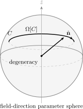
The direction $\hat{\mathbf n}$ traces a closed loop $C$ on the fixed-gap parameter sphere. For the Hamiltonian and eigenstate convention above, the Berry phase is minus one half of the oriented solid angle $\Omega[C]$.

Three lessons are packed into this example.

First, the sign is conventional until the Hamiltonian, eigenstate, loop orientation, and curvature orientation are fixed. Second, the phase is geometric: changing the loop shape changes its enclosed solid angle continuously. Third, the full-sphere curvature flux is quantized:

$$\frac{1}{2\pi} \int_{S^2}F_+ = -1.$$

The sphere surrounds the degeneracy at $\Delta=0$. The local solid-angle phase and the global Chern number are different views of the same eigenline geometry.

Local Gauges and Global Patching

A local eigenvector can be perfectly smooth even when no smooth global eigenvector exists. On overlapping patches $U_\alpha$ and $U_\beta$,

$$|n_\beta\rangle = e^{i\chi_{\beta\alpha}} |n_\alpha\rangle,$$

so

$$A_\beta = A_\alpha-d\chi_{\beta\alpha}.$$

The curvature agrees on the overlap:

$$F_\beta=F_\alpha.$$

Global information is then carried by the winding of the transition phase. This resolves an apparent paradox. A locally real eigenvector may have $A=0$ on every chosen patch, yet the transition functions can still produce a sign change or nontrivial loop phase.

The molecular phase around a conical intersection is a standard example. An electronic eigenvector can be chosen real locally, but it can return with a minus sign after one circuit. The local connection vanishes in the real gauges; the global patching carries the phase $\pi$.

Geometric Does Not Mean Topological

The words describe different levels of structure.

Property	Geometric quantity	Topological quantity
typical example	Berry phase $\gamma[C]$	Chern number $C$
response to smooth path deformation	can vary continuously	remains fixed inside the defining class
local input	connection or curvature	global patching or integrated curvature
usual value set	continuous modulo $2\pi$	discrete, often integer
protection assumptions	well-defined transport	gap, smooth bundle, closed base, and sometimes symmetry

A generic Berry phase is geometric and path dependent. It becomes topological only when additional structure prevents continuous change, for example:

• the loop cannot be contracted without crossing an excluded region or degeneracy;
• a symmetry quantizes the phase to $0$ or $\pi$ modulo $2\pi$;
• the phase is related to an integer curvature integral on a closed surface;
• the relevant map has a nonzero winding number.

Conversely, curvature itself need not be quantized. Its distribution can move continuously while its properly normalized integral stays fixed.

Chern Numbers

Let $M$ be a closed oriented two-dimensional parameter space, and suppose an eigenstate line is isolated over all of $M$. Its first Chern number is

$$C_n = \frac{1}{2\pi} \int_M F_n.$$

Under the stated assumptions,

$$C_n\in\mathbb Z.$$

The integer arises from patching. If one global smooth potential $A_n$ existed on a closed $M$, then

$$\int_MF_n = \int_MdA_n = \int_{\partial M}A_n = 0.$$

Therefore a nonzero Chern number obstructs one smooth global eigenvector gauge. Local gauges remain valid; they simply require transition functions with nonzero winding.

A Chern number can change only when the defining family leaves its admissible class. In an energy-band problem this normally requires a gap closing, at which point the occupied bundle being tracked is no longer isolated.

Berry and Aharonov–Bohm Holonomy

The two effects share a mathematical pattern:

$$\text{connection} \quad\longrightarrow\quad \text{closed-loop phase}.$$

Their physical data are different.

Feature	Berry phase	Aharonov–Bohm phase
base space	Hamiltonian parameter space	particle configuration space
connection	$A_n=i\langle n	dn\rangle$
loop	path of an eigenspace	particle path around flux
central assumption	adiabatic following in the standard Berry setup	coherent charged-particle propagation
phase	$\oint_C A_n$	$(q/\hbar)\oint_C\mathbf A\cdot d\mathbf r$
source or obstruction	degeneracy or twisted eigenbundle	magnetic flux or excluded region

In the ideal Aharonov–Bohm setup,

$$\Delta\varphi_{\mathrm{AB}} = \frac{q}{\hbar} \oint_C \mathbf A\cdot d\mathbf r = \frac{q\Phi}{\hbar}.$$

No slow variation of a Hamiltonian parameter is required in that basic description. It is therefore better to call Berry and Aharonov–Bohm phases related holonomies than to declare them identical effects.

Born–Oppenheimer Geometry

For a molecular Hamiltonian

$$H_{\mathrm{mol}} = T_N+H_e(r;R),$$

the nuclear coordinates $R$ act as parameters for the electronic problem

$$H_e(R)|\phi_a(R)\rangle = E_a(R)|\phi_a(R)\rangle.$$

An isolated electronic state defines the molecular Berry connection

$$\mathbf A_a(R) = i \langle\phi_a(R)| \nabla_R\phi_a(R)\rangle_e.$$

The effective nuclear momentum becomes

$$-i\hbar\nabla_R \longmapsto -i\hbar\nabla_R - \hbar\mathbf A_a(R).$$

This connection is not an externally applied electromagnetic potential. It is induced by the $R$-dependence of the electronic eigenstate. Around a conical intersection, a closed nuclear path can acquire

$$\gamma_a[C] = \pi \quad \operatorname{mod}2\pi.$$

The same region also enhances off-diagonal nonadiabatic couplings because the electronic gap becomes small. A one-surface Berry phase applies to a loop that avoids the degeneracy; dynamics through the degeneracy generally requires a multi-surface treatment.

Momentum-Space Geometry

For a one-dimensional isolated Bloch band, crystal momentum lives on a circle:

$$\mathrm{BZ}\simeq S^1.$$

With cell-periodic states $|u_{nk}\rangle$, the Zak phase is

$$\gamma_n = \oint_{\mathrm{BZ}} i\langle u_{nk}|\partial_k u_{nk}\rangle\,dk \quad \operatorname{mod}2\pi.$$

If the chosen gauge is not periodic, an endpoint-overlap term must be included. The raw Zak phase can also depend on origin, unit-cell, and orbital conventions. Symmetry can quantize it, but one must state the protecting symmetry and the occupied subspace.

For a two-dimensional isolated Bloch band,

$$\mathrm{BZ}\simeq T^2,$$

and the natural global invariant is a Chern number:

$$C_n = \frac{1}{2\pi} \int_{\mathrm{BZ}}F_n.$$

In the clean noninteracting filled-band setting,

$$\sigma_{xy} = \frac{e^2}{h} C_{\mathrm{occ}},$$

up to charge-sign and orientation conventions. This formula is a bridge, not the whole quantum Hall effect. Plateau formation also involves disorder and localization; fractional Hall states require interacting many-body topology.

Boundary Twists and Many-Body Geometry

Berry geometry is not restricted to single-particle bands. Put a many-body system on a torus and impose boundary twists

$$(\theta_x,\theta_y) \in T^2.$$

If the ground state remains nondegenerate and gapped over this twist torus, it defines a Berry curvature

$$F_{\theta_x\theta_y} = \partial_{\theta_x}A_{\theta_y} - \partial_{\theta_y}A_{\theta_x}.$$

The corresponding Chern number is

$$C = \frac{1}{2\pi} \int_0^{2\pi} \int_0^{2\pi} F_{\theta_x\theta_y} \,d\theta_x\,d\theta_y.$$

This example clarifies the role of parameter space. The two-dimensional base need not be physical real space or a Brillouin zone; it can be a space of boundary conditions.

Degenerate Subspaces and Non-Abelian Holonomy

Suppose an $N$-dimensional eigenspace remains degenerate and separated by a gap from all other states. Choose a local orthonormal frame

$$|u_a(R)\rangle, \qquad a=1,\ldots,N.$$

The frame may be changed by $G(R)\in U(N)$:

$$|u_a'\rangle = \sum_b |u_b\rangle G_{ba}.$$

The matrix Berry connection is

$$(A)_{ab} = i\langle u_a|du_b\rangle.$$

Adiabatic transport gives the Wilczek–Zee holonomy

$$\mathcal U_{\mathrm{WZ}}[C] = \mathcal P \exp \left( i\int_C A \right).$$

Path ordering is essential because matrices at different points need not commute. Under a frame change,

$$A' = G^{-1}AG + iG^{-1}dG,$$

and a closed-loop holonomy based at $R_0$ transforms by conjugation:

$$\mathcal U_{\mathrm{WZ}}[C] \longmapsto G(R_0)^{-1} \mathcal U_{\mathrm{WZ}}[C] G(R_0).$$

The matrix depends on the chosen base-point frame, while its eigenvalues and trace-type conjugacy data are gauge invariant. This is geometric rotation within an isolated subspace, not leakage out of that subspace and not a dynamical nonabelian gauge field.

A Reliable Geometry Workflow

1. Identify the base space

State what the parameters are and which loops or surfaces are physically available. Do not silently replace parameter space with physical space.

2. Identify the isolated object

Decide whether the relevant object is one nondegenerate eigenline, an occupied multi-band subspace, or a degenerate eigenspace. Check the gap on the entire region used.

3. Fix conventions

State the Hamiltonian sign, eigenstate label, loop orientation, and connection convention. Here,

$$A=i\langle n|dn\rangle, \qquad A\mapsto A-d\chi.$$

4. Compute local data

Use eigenvectors for analytic work or projectors for gauge-stable formulas. If numerical eigenvectors have arbitrary phases, use overlap or Wilson-loop methods rather than differentiating a discontinuous gauge blindly.

5. Form the invariant quantity

For a closed path, compute holonomy. For a small loop, curvature flux may be simplest. For a closed two-dimensional base, test whether a Chern number is defined.

6. Inspect singularities and patches

Locate level crossings, excluded regions, and gauge singularities. Distinguish a bad coordinate gauge from a genuine closing of the spectral gap.

7. State the protection assumptions

If a quantity is called topological, name the gap, symmetry, smoothness, orientation, and boundary conditions that define its deformation class.

8. Connect to an observable

Phases require interference or a relative comparison. Curvature enters response only through a physical formula with occupation and dynamical assumptions. A Chern number is not by itself a complete transport experiment.

9. Respect the canonical boundary

Use this chapter for geometric structure. Follow the links to dynamics, molecular physics, quantum matter, quantum information, or QFT for the complete application.

Chapter Map

Foundations

1. Begin with Dynamical Phase versus Geometric Phase to separate the two contributions to cyclic phase.
2. Read Adiabatic Theorem Reminder before applying an instantaneous-eigenstate formula.
3. Use Berry Phase for the standard cyclic setup.

Local and global geometry

1. Berry Connection introduces local gauge data.
2. Parallel Transport turns the connection into a transport rule.
3. Holonomy explains the finite closed-loop mismatch.
4. Berry Curvature measures infinitesimal-loop phase and identifies degeneracies as curvature sources.

Canonical examples

1. Berry Phase for Spin-1/2 gives the solid-angle derivation.
2. Berry Phase in the Aharonov–Bohm Effect compares parameter-space and real-space holonomy.
3. Born–Oppenheimer Berry Phase applies the construction to nuclear-coordinate space.

Topology and quantum matter

1. Chern Numbers explains quantized curvature flux.
2. Zak Phase Preview treats one-dimensional Brillouin-zone holonomy.
3. Quantum Hall Geometry Preview connects Chern number to Hall response.
4. Topological Quantum Numbers clarifies what deformation-stable labels do and do not mean.
5. Non-Abelian Berry Phase Preview extends transport to isolated degenerate subspaces.

Reading Paths

First graduate pass

Dynamical versus Geometric Phase → Adiabatic Theorem Reminder → Berry Phase → Berry Connection → Berry Curvature → Spin-1/2 Example.

Geometry and topology

Parallel Transport → Holonomy → Chern Numbers → Topological Quantum Numbers.

Molecular physics

Adiabatic Theorem Reminder → Berry Connection → Born–Oppenheimer Berry Phase.

Quantum matter

Berry Curvature → Chern Numbers → Zak Phase Preview → Quantum Hall Geometry Preview.

Degenerate transport

Holonomy → Non-Abelian Berry Phase Preview → From Berry Phase to Topological Terms.

Distinctions Worth Keeping

Do not identify	Reason
total phase and Berry phase	the total phase generally also contains a dynamical contribution
cyclic controls and adiabatic evolution	a Hamiltonian can return to itself while the state undergoes nonadiabatic transitions
ket and ray	a ket may change phase while the physical pure state is unchanged
connection and curvature	the connection is gauge dependent; abelian curvature is gauge invariant
local flatness and trivial holonomy	noncontractible loops can carry holonomy even where local curvature vanishes
geometric and topological	geometric phases can vary continuously; topological invariants require stronger hypotheses
gauge singularity and physical degeneracy	a gauge pole can be moved between patches; a level crossing is spectral
Berry and Aharonov–Bohm connections	one is induced by an eigenstate family, the other is electromagnetic
individual bands and occupied subspace	mixed occupied bands may have only a collective invariant
non-Abelian holonomy and gauge-field dynamics	matrix transport in a degenerate subspace does not by itself define Yang–Mills dynamics

Common Mistakes

• Calling every cyclic phase a Berry phase.
• Applying the nondegenerate formula through a level crossing.
• Quoting $\gamma=-\Omega/2$ without fixing Hamiltonian, eigenstate, and orientation conventions.
• Treating the Berry connection as directly gauge invariant.
• Using an open-path connection integral without an endpoint comparison.
• Assuming a locally real eigenvector rules out global geometric phase.
• Calling any Berry phase topological.
• Integrating curvature over an open patch and calling the result a Chern number.
• Forgetting that a Chern number needs a closed base and an isolated bundle over the entire base.
• Ignoring unit-cell and origin conventions in a Zak phase.
• Assigning separate invariants to bands that mix within an isolated occupied subspace.
• Treating quantized Hall response as a consequence of topology alone, without the filling, gap, response, and localization assumptions of the physical setting.

Cross-Links

• Projective Hilbert Space
• Time-Dependent Hamiltonians
• Adiabatic Theorem
• Adiabatic Approximation as a Method
• Gauge, Phase, and Magnetic Geometry
• Aharonov–Bohm Effect
• Dirac Monopole Preview
• Differential Forms
• Connections and Curvature
• Parallel Transport
• Holonomy
• U(1) Bundles and Quantum Phase
• Berry Connection as a Mathematical Object
• Chern Numbers
• Topological Invariants
• Born–Oppenheimer Approximation as Scale Separation
• Landau Levels
• Berry Phase Problems
• Symmetry Breaking and Emergence
• From Berry Phase to Topological Terms

References

• S. Pancharatnam, “Generalized theory of interference, and its applications,” Proceedings of the Indian Academy of Sciences A 44, 247–262, 1956.
• Y. Aharonov and D. Bohm, “Significance of electromagnetic potentials in the quantum theory,” Physical Review 115, 485–491, 1959.
• C. A. Mead and D. G. Truhlar, “On the determination of Born–Oppenheimer nuclear motion wave functions including complications due to conical intersections and identical nuclei,” Journal of Chemical Physics 70, 2284–2296, 1979.
• D. J. Thouless, M. Kohmoto, M. P. Nightingale, and M. den Nijs, “Quantized Hall conductance in a two-dimensional periodic potential,” Physical Review Letters 49, 405–408, 1982.
• B. Simon, “Holonomy, the quantum adiabatic theorem, and Berry’s phase,” Physical Review Letters 51, 2167–2170, 1983.
• M. V. Berry, “Quantal phase factors accompanying adiabatic changes,” Proceedings of the Royal Society A 392, 45–57, 1984.
• F. Wilczek and A. Zee, “Appearance of gauge structure in simple dynamical systems,” Physical Review Letters 52, 2111–2114, 1984.
• Y. Aharonov and J. Anandan, “Phase change during a cyclic quantum evolution,” Physical Review Letters 58, 1593–1596, 1987.
• A. Shapere and F. Wilczek, eds., Geometric Phases in Physics, World Scientific, 1989.
• J. Zak, “Berry’s phase for energy bands in solids,” Physical Review Letters 62, 2747–2750, 1989.
• C. A. Mead, “The geometric phase in molecular systems,” Reviews of Modern Physics 64, 51–85, 1992.
• D. Vanderbilt, Berry Phases in Electronic Structure Theory, Cambridge University Press, 2018.

Exercises

1. Starting from $A=i\langle n|dn\rangle$, derive the gauge transformation of the connection under $|n\rangle\mapsto e^{i\chi}|n\rangle$. Then show directly that $F=dA$ is gauge invariant.

Solution

The transformed connection is

$$\begin{aligned} A' &= i \langle n| e^{-i\chi} d \left( e^{i\chi}|n\rangle \right) \\ &= i \left( i\,d\chi + \langle n|dn\rangle \right) \\ &= A-d\chi. \end{aligned}$$

Taking an exterior derivative,

$$F' = dA' = dA-d^2\chi = F,$$

because $d^2=0$.

2. A closed parameter path is traversed once in time $T$ and again in time $2T$, with the same energy $E_n$ at each corresponding point of the path. Assume both protocols are adiabatic. Compare their dynamical and Berry phases.

Solution

If the second protocol uses the same path at half the speed, then it spends twice as long at each energy. Therefore

$$\alpha_{\mathrm{dyn}}(2T) = 2\alpha_{\mathrm{dyn}}(T).$$

The Berry phase is the line integral of a one-form over the oriented path:

$$\gamma[C] = \oint_C A.$$

It is invariant under an orientation-preserving reparameterization, so

$$\gamma_{2T}[C] = \gamma_T[C].$$

The conclusion depends on both traversals remaining adiabatic. Reversing the path orientation would instead reverse the Berry phase.

3. For the spin-$1/2$ convention in this page, let the field direction follow a circle of fixed polar angle $\theta_0$ with $\phi:0\to2\pi$. Find the Berry phase and its limiting values at $\theta_0=0$ and $\theta_0=\pi/2$.

Solution

The enclosed solid angle is

$$\Omega = 2\pi \left( 1-\cos\theta_0 \right).$$

Hence

$$\gamma_+ = -\frac{\Omega}{2} = -\pi \left( 1-\cos\theta_0 \right) \quad \operatorname{mod}2\pi.$$

At the north pole, $\theta_0=0$, the loop shrinks and $\gamma_+=0$. At the equator, $\theta_0=\pi/2$, the phase is $-\pi$, equivalent to $\pi$ modulo $2\pi$.

4. Integrate

$$F_+ = -\frac12 \sin\theta\,d\theta\wedge d\phi$$

over the standard oriented sphere and compute the Chern number. Which assumptions make the result meaningful?

Solution

Using $0\le\theta\le\pi$ and $0\le\phi<2\pi$,

$$\begin{aligned} \int_{S^2}F_+ &= -\frac12 \int_0^{2\pi}d\phi \int_0^\pi \sin\theta\,d\theta \\ &= -2\pi. \end{aligned}$$

Therefore

$$C_+ = \frac{1}{2\pi} \int_{S^2}F_+ = -1.$$

The sphere must be closed and oriented, and the chosen eigenstate must remain isolated at every point on the sphere. The degeneracy may lie inside the sphere, but not on it.

5. Classify each statement as geometric, topological under stated conditions, or neither:

   (a) a Berry phase that changes continuously when a contractible loop is deformed;

   (b) a filled-band Chern number while the occupied gap remains open;

   (c) the raw integral of a numerically discontinuous Berry connection along an open path;

   (d) a Zak phase restricted to $0$ or $\pi$ by an unbroken protecting symmetry.

Solution

(a) is geometric but not topological. Its path dependence is precisely geometric information.

(b) is topological under the gap and bundle assumptions. It cannot change continuously while the occupied subspace remains isolated.

(c) is neither a well-defined gauge-invariant geometric observable nor a topological invariant. An open-path phase needs endpoint data, and a discontinuous numerical gauge must be handled with overlap or Wilson-line methods.

(d) is topological or symmetry-protected within the class that preserves the relevant symmetry, gap, and conventions. Breaking the protecting symmetry can remove the quantization without contradicting topology.

6. In a two-dimensional degenerate eigenspace, suppose the connection along the first half of a path is proportional to $\sigma_x$ and along the second half is proportional to $\sigma_y$. Explain why reversing the order can change the holonomy.

Solution

Let the two segment transports be

$$U_x=e^{i\alpha\sigma_x}, \qquad U_y=e^{i\beta\sigma_y}.$$

Traversing the $x$ segment and then the $y$ segment gives

$$U_{yx} = U_yU_x,$$

whereas the reversed ordering gives

$$U_{xy} = U_xU_y.$$

Because

$$[\sigma_x,\sigma_y] = 2i\sigma_z,$$

the two products are generally unequal. The path-ordered exponential records this physical ordering. In the one-dimensional abelian case the connection values commute, so this particular ordering issue disappears.