Adiabatic Approximation as a Method

The adiabatic approximation is a method for evolving states under a Hamiltonian whose eigenspaces change slowly. One first diagonalizes the instantaneous Hamiltonian, then estimates couplings generated by the moving basis, chooses a runtime or schedule that suppresses leakage, and finally tracks the phases accumulated by the followed eigenspaces.

This page owns that calculational workflow and its leading corrections. The concise theorem statement belongs in the Adiabatic Theorem reference card. The phase split needed for geometric phases is reviewed in Adiabatic Theorem Reminder. Berry connection, curvature, holonomy, and topology remain canonical in Berry Phase and its neighboring geometry pages.

Put the Protocol on a Fixed Interval

Write a protocol of total duration $T$ using dimensionless time

$$s \equiv \frac{t}{T}, \qquad 0\le s\le1.$$

The Hamiltonian is

$$H_T(t) = H(s).$$

Increasing $T$ traverses the same path $H(s)$ more slowly. This separation is essential: it distinguishes the geometric path through Hamiltonian space from the rate at which that path is followed.

At each $s$, solve

$$H(s)\lvert n(s)\rangle = E_n(s)\lvert n(s)\rangle.$$

For a nondegenerate target level $n$, define the instantaneous gaps

$$\Delta_{mn}(s) \equiv E_m(s)-E_n(s)$$

and the minimum target gap

$$\begin{aligned} g(s) &\equiv \min_{m\ne n} \left\lvert \Delta_{mn}(s) \right\rvert, \\ g_{\min} &\equiv \min_{s\in[0,1]}g(s). \end{aligned}$$

The elementary gapped method assumes

$$g_{\min}\gt0.$$

The label $n$ should follow a continuous eigenbranch or isolated spectral subspace, not merely “the third-lowest eigenvalue” if level ordering changes.

What the Approximation Predicts

If the system starts in $\lvert n(0)\rangle$ and the protocol is adiabatic, then

$$\begin{aligned} \lvert\psi_{\mathrm{ad}}(t)\rangle &= e^{i\gamma_n(t)} \exp\left[ -\frac{i}{\hbar} \int_0^tE_n(t')\,dt' \right] \\ &\quad\times \lvert n(t)\rangle. \end{aligned}$$

The dynamical phase is

$$\delta_n(t) = -\frac{1}{\hbar} \int_0^tE_n(t')\,dt',$$

while, in a chosen smooth gauge, the geometric contribution is

$$\gamma_n(t) = i \int_0^t \langle n(t')\vert\dot n(t')\rangle\,dt'.$$

Adiabatic following means that population remains near the corresponding instantaneous eigenspace. It does not mean that the ket is constant. The eigenspace moves, the dynamical phase grows with runtime, and geometric transport can contribute an additional phase.

For final energy populations, an overall phase is irrelevant. For interferometry, coherent superpositions, cyclic evolution, or later recombination, relative dynamical and geometric phases are observable and must be retained. Their gauge structure and closed-loop interpretation belong in the geometry volume.

Exact Equations in the Instantaneous Basis

Choose a smooth local phase convention satisfying

$$\langle n(s)\vert \partial_s n(s)\rangle = 0.$$

This is the parallel-transport gauge along the open interval. Expand the exact state as

$$\begin{aligned} \lvert\psi(s)\rangle &= \sum_k a_k(s) \\ &\qquad\times \exp\left[ -\frac{iT}{\hbar} \int_0^sE_k(u)\,du \right] \\ &\qquad\times \lvert k(s)\rangle. \end{aligned}$$

Substituting into the Schrödinger equation gives

$$\begin{aligned} \partial_s a_m(s) &= - \sum_{k\ne m} a_k(s) \langle m(s)\vert \partial_s k(s)\rangle \\ &\qquad\times \exp\left[ \frac{iT}{\hbar} \int_0^s \Delta_{mk}(u)\,du \right]. \end{aligned}$$

This equation contains the whole mechanism:

• the moving eigenbasis generates off-diagonal couplings $\langle m\vert\partial_s k\rangle$;
• the accumulated gap generates a rapidly oscillating phase;
• slow evolution means that destructive interference suppresses net transfer between separated eigenspaces.

The approximation is therefore not based only on a small instantaneous coupling. Oscillatory cancellation, endpoints, smoothness, and the full path all matter.

Replace Eigenvector Derivatives by Hamiltonian Derivatives

Differentiate

$$H(s)\lvert n(s)\rangle = E_n(s)\lvert n(s)\rangle$$

and project onto $\langle m(s)\rvert$ with $m\ne n$. One obtains

$$\langle m\vert \partial_s n\rangle = \frac{ \langle m\vert \partial_sH \lvert n\rangle }{ E_n-E_m }.$$

In physical time,

$$\dot H(t) = \frac{1}{T} \partial_sH(s).$$

The familiar pairwise diagnostic is therefore

$$\eta_{mn}(s) \equiv \frac{ \hbar \left\lvert \langle m(s)\vert \dot H(t) \lvert n(s)\rangle \right\rvert }{ \left\lvert \Delta_{mn}(s) \right\rvert^2 } \ll1.$$

Equivalently,

$$\eta_{mn}(s) = \frac{\hbar}{T} \frac{ \left\lvert \langle m(s)\vert \partial_sH(s) \lvert n(s)\rangle \right\rvert }{ \left\lvert \Delta_{mn}(s) \right\rvert^2 }.$$

A conservative runtime estimate is

$$T \gg \hbar \max_{\substack{s\in[0,1]\\m\ne n}} \frac{ \left\lvert \langle m(s)\vert \partial_sH(s) \lvert n(s)\rangle \right\rvert }{ \left\lvert \Delta_{mn}(s) \right\rvert^2 }.$$

This estimate has the right dimensions and exposes the squared gap. It is a diagnostic, not a theorem by itself. It can be overly pessimistic, and a small pointwise ratio does not automatically control endpoint effects, rapidly changing derivatives, long sums over states, unbounded domains, or many-body limits.

Leading Nonadiabatic Amplitude

Suppose

$$a_n(0)=1, \qquad a_m(0)=0 \quad (m\ne n).$$

Keeping the target amplitude fixed at leading order gives

$$\begin{aligned} a_m^{(1)}(1) &= - \int_0^1ds\, \langle m(s)\vert \partial_s n(s)\rangle \\ &\qquad\times \exp\left[ iT \int_0^s \omega_{mn}(u)\,du \right], \end{aligned}$$

where

$$\omega_{mn}(s) \equiv \frac{\Delta_{mn}(s)}{\hbar}.$$

This formula is adiabatic perturbation theory at first order. It keeps the entire path and phase history, unlike a local maximum criterion.

Define

$$f_{mn}(s) \equiv \langle m(s)\vert \partial_s n(s)\rangle$$

and

$$\Theta_{mn}(s) \equiv \int_0^s\omega_{mn}(u)\,du.$$

When $\omega_{mn}$ never vanishes, integration by parts gives

$$\begin{aligned} a_m^{(1)}(1) &= - \left[ \frac{ f_{mn}(s) e^{iT\Theta_{mn}(s)} }{ iT\omega_{mn}(s) } \right]_{0}^{1} \\ &\quad+ \frac{1}{iT} \int_0^1ds\, e^{iT\Theta_{mn}(s)} \\ &\qquad\times \partial_s \left( \frac{f_{mn}(s)}{\omega_{mn}(s)} \right). \end{aligned}$$

The explicit factor $1/T$ explains the generic scaling

$$a_m^{(1)} = O(T^{-1}), \qquad P_{m\leftarrow n} = O(T^{-2}).$$

It also reveals two facts hidden by the pointwise diagnostic:

1. boundary terms can dominate;
2. derivatives of couplings and gaps enter the remainder.

A Schematic Leakage Bound

For a smooth finite-dimensional Hamiltonian with a nondegenerate target level and gap $g(s)\ge g_{\min}\gt0$, a representative bound has the structure

$$\begin{aligned} \epsilon_{\mathrm{leak}} \lesssim \frac{\hbar}{T} \Bigg[ & \frac{ \lVert\partial_sH(0)\rVert }{ g^2(0) } \\ &\quad+ \frac{ \lVert\partial_sH(1)\rVert }{ g^2(1) } \\ &+ \int_0^1ds\, \frac{ \lVert\partial_s^2H\rVert }{ g^2 } \\ &\quad+ \int_0^1ds\, \frac{ \lVert\partial_sH\rVert^2 }{ g^3 } \Bigg]. \end{aligned}$$

Here $\epsilon_{\mathrm{leak}}$ denotes a norm of the component outside the followed eigenspace, and omitted numerical constants depend on the precise theorem and norm. This is a scaling template, not a universal bound for all Hamiltonians. Its purpose is to show why the minimum gap alone is insufficient: endpoint derivatives and path smoothness also enter.

For unbounded operators, changing domains, continuous spectra, or many-body thermodynamic limits, one must use a theorem suited to the problem rather than substituting formal operator norms.

Boundary Cancellation and Smooth Schedules

If the protocol begins and ends smoothly,

$$\partial_sH(0) = \partial_sH(1) = 0,$$

then the leading boundary term often vanishes. With a nonclosing gap and sufficient differentiability, a second integration by parts can improve the leading transition amplitude to

$$a_m = O(T^{-2}).$$

Higher-order endpoint cancellation can produce further algebraic improvement when the required derivatives vanish and the Hamiltonian remains smooth. This does not mean that every smooth-looking schedule is exponentially accurate. The result depends on differentiability, analytic structure, gap behavior, and how the protocol is switched.

The practical lesson is simple: avoid abruptly turning a supposedly adiabatic protocol on or off.

Local Adiabatic Scheduling

Suppose the Hamiltonian depends on one control $\lambda$:

$$H=H(\lambda).$$

Then

$$\dot H = \dot\lambda\, \partial_\lambda H.$$

A local speed budget for the target level is

$$\left\lvert\dot\lambda\right\rvert \ll \min_{m\ne n} \frac{ \left\lvert\Delta_{mn}(\lambda)\right\rvert^2 }{ \hbar \left\lvert \langle m(\lambda)\vert \partial_\lambda H \lvert n(\lambda)\rangle \right\rvert }.$$

One may choose a schedule that moves rapidly where gaps are large and slows near a small avoided crossing. Holding a chosen local diagnostic near a small constant $\eta_0$ gives

$$\left\lvert\dot\lambda\right\rvert = \eta_0 \min_{m\ne n} \frac{ \left\lvert\Delta_{mn}(\lambda)\right\rvert^2 }{ \hbar \left\lvert \langle m(\lambda)\vert \partial_\lambda H \lvert n(\lambda)\rangle \right\rvert }.$$

The resulting runtime is

$$T = \int_{\lambda_i}^{\lambda_f} \frac{d\lambda}{ \left\lvert\dot\lambda\right\rvert }.$$

This local schedule is a design heuristic. The integrated transition amplitude and endpoint smoothness still need to be checked.

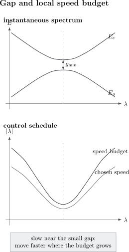
The energy gap is smallest near an avoided crossing. A local adiabatic schedule lowers the control speed in that region and uses a larger speed where the gap and transition budget permit it. The matrix element of $\partial_\lambda H$, not the gap alone, determines the allowed speed.

Worked Example: A Rotating Two-Level Hamiltonian

Consider

$$\begin{aligned} H(t) &= -\frac{\hbar\omega_0}{2} \cos\theta(t)\,\sigma_z \\ &\quad- \frac{\hbar\omega_0}{2} \sin\theta(t)\,\sigma_x, \\ \omega_0 &\gt 0. \end{aligned}$$

The instantaneous gap is constant:

$$\Delta_{eg} = \hbar\omega_0.$$

Choose real instantaneous eigenvectors. Their off-diagonal derivative coupling has magnitude

$$\left\lvert \langle e(t)\vert\dot g(t)\rangle \right\rvert = \frac{ \left\lvert\dot\theta(t)\right\rvert }{2}.$$

The local diagnostic is

$$\frac{ \left\lvert\dot\theta(t)\right\rvert }{ 2\omega_0 } \ll1.$$

For a constant angular speed

$$\dot\theta = \Omega$$

over a duration $T$, first-order adiabatic perturbation theory gives

$$\begin{aligned} a_e^{(1)}(T) &= - \frac{\Omega}{2} \int_0^T e^{i\omega_0t}\,dt \\ &= - \frac{\Omega}{ 2i\omega_0 } \left( e^{i\omega_0T}-1 \right). \end{aligned}$$

Hence

$$P_{e\leftarrow g}^{(1)} = \frac{\Omega^2}{\omega_0^2} \sin^2\left( \frac{\omega_0T}{2} \right).$$

The probability is bounded by

$$P_{e\leftarrow g}^{(1)} \le \left( \frac{\Omega}{\omega_0} \right)^2.$$

This example shows both the expected small parameter and the oscillatory cancellation missed by a worst-case local estimate. If the rotation is switched on and off abruptly, its endpoint terms remain visible. A smooth $\dot\theta(t)$ can suppress them.

Example: A Locally Scheduled Avoided Crossing

Use

$$H(\lambda) = \frac12 \left( \lambda\,\sigma_z + g\,\sigma_x \right), \qquad g\gt0.$$

The gap is

$$\Delta(\lambda) = \sqrt{\lambda^2+g^2},$$

and

$$\left\lvert \langle e\vert \partial_\lambda H \lvert g\rangle \right\rvert = \frac{ g }{ 2\sqrt{\lambda^2+g^2} }.$$

Holding the pairwise diagnostic at $\eta_0$ gives

$$\left\lvert\dot\lambda\right\rvert = \frac{ 2\eta_0 \left( \lambda^2+g^2 \right)^{3/2} }{ \hbar g }.$$

For a symmetric sweep from $-\Lambda$ to $+\Lambda$,

$$\begin{aligned} T &= \frac{\hbar g}{2\eta_0} \int_{-\Lambda}^{\Lambda} \frac{d\lambda}{ (\lambda^2+g^2)^{3/2} } \\ &= \frac{ \hbar\Lambda }{ \eta_0g \sqrt{\Lambda^2+g^2} }. \end{aligned}$$

When $\Lambda\gg g$,

$$T \simeq \frac{\hbar}{ \eta_0g }.$$

This improves on applying the minimum-gap speed limit uniformly over the entire range. It does not replace the exact Landau–Zener Transition result for a specified linear sweep.

Degenerate Eigenspaces and Projector Transport

Internal degeneracy does not automatically destroy adiabatic following. Let $P(s)$ project onto a possibly degenerate spectral cluster separated from the rest of the spectrum by a nonzero gap. The adiabatic statement is that the evolved state remains close to

$$\operatorname{Ran}P(s).$$

Kato’s adiabatic Hamiltonian is

$$H_{\mathrm A}(t) = H(t) + i\hbar \left[ \dot P(t),P(t) \right].$$

Its evolution intertwines the projectors:

$$U_{\mathrm A}(t)P(0) U_{\mathrm A}^\dagger(t) = P(t).$$

Indeed,

$$\left[ \left[ \dot P,P \right], P \right] = \dot P,$$

which follows from differentiating $P^2=P$. The commutator term transports the subspace while the block of $H$ supplies dynamical evolution inside it.

For a one-dimensional eigenspace this reduces to phase transport. For a degenerate cluster, evolution within the subspace can be matrix valued. The non-Abelian connection and its geometric interpretation belong in Non-Abelian Berry Phase Preview.

Crossings and Labeling

At a true gap closing,

$$g_{\min}=0,$$

the elementary isolated-eigenspace argument fails. Several distinct situations must be separated:

• an avoided crossing has a small but nonzero gap and may require a long runtime;
• an exact crossing protected by symmetry can preserve a symmetry sector even though globally ordered energy labels cross;
• an accidental or symmetry-breaking crossing can mix the target with another state;
• a continuum threshold can destroy the finite-dimensional gap picture entirely.

Near an isolated avoided crossing, reduce to the relevant low-energy subspace when justified and use Landau–Zener or direct propagation. Do not hide a closing gap by relabeling eigenvalues.

Superpositions and Mixed States

If the initial state is a superposition,

$$\lvert\psi(0)\rangle = \sum_n c_n\lvert n(0)\rangle,$$

and each occupied branch remains isolated, then

$$\begin{aligned} \lvert\psi_{\mathrm{ad}}(t)\rangle &= \sum_n c_n e^{i\gamma_n(t)} \\ &\qquad\times \exp\left[ -\frac{i}{\hbar} \int_0^tE_n(t')\,dt' \right] \\ &\qquad\times \lvert n(t)\rangle. \end{aligned}$$

Relative phases can change interference even when every branch has negligible leakage. Population fidelity alone is therefore not a complete error metric.

For an initial density operator diagonal in isolated projectors,

$$\rho(0) = \sum_n p_nP_n(0),$$

adiabatic evolution transports each population to the corresponding final projector, up to leakage and any internal unitary dynamics in degenerate blocks. Coherences require phase-sensitive tracking.

Applications and Boundaries

Molecular separation of scales

In Born–Oppenheimer reasoning, nuclear coordinates $\mathbf R(t)$ vary slowly compared with electronic dynamics. Electronic derivative couplings have the form

$$\mathbf d_{mn}(\mathbf R) \equiv \langle m(\mathbf R)\vert \nabla_{\mathbf R}n(\mathbf R)\rangle,$$

and nuclear motion drives transitions through

$$\dot{\mathbf R} \cdot \mathbf d_{mn}(\mathbf R).$$

Large electronic gaps and slow nuclear velocities suppress transitions between electronic surfaces. The exact channel equations, mass scaling, and wavepacket-level diagnostics are developed in Born–Oppenheimer Approximation as Scale Separation. Conical intersections and near-degeneracies invalidate a single-surface approximation and can generate geometric effects; the latter belong in Born–Oppenheimer Berry Phase.

Adiabatic state preparation

Choose $H(0)$ with an accessible eigenstate and a path to a target Hamiltonian $H(1)$. If the followed spectral subspace stays gapped and the runtime is sufficient, the protocol prepares the corresponding final eigenstate. A useful design must report the path, gap, coupling matrix elements, schedule, endpoint smoothness, and target error.

Adiabatic quantum computing preview

Adiabatic quantum computation encodes a problem in a final Hamiltonian and begins from an easily prepared ground state. Its performance depends on the gap along the interpolation, matrix elements of the driving term, schedule choice, precision, noise, and how these quantities scale with problem size. The slogan “runtime is inverse gap squared” is only a rough worst-case guide, not a complete complexity statement. Adiabatic Quantum Computation owns the corresponding computation-model record: instance encoding, accepted ground subspace and decoder, uniform Hamiltonian path, declared schedule and error certificate, circuit equivalence, and normalized logical resources; this page retains the general instantaneous-eigenspace and leakage calculation.

Quantum control

Slow passage can transfer population robustly when the desired eigenbranch is isolated. Real protocols balance adiabatic leakage against decoherence, control noise, and finite experimental time. In an open system, a closed-system adiabatic theorem is not automatically the right approximation.

Relation to Sudden and Landau–Zener Limits

The Sudden Approximation holds the state vector nearly fixed while the Hamiltonian basis changes. The adiabatic approximation instead transports the state with an instantaneous eigenspace. These are opposite controlled limits of a protocol family.

Landau–Zener dynamics resolves a standard intermediate problem. It gives an exact transition probability for an ideal linear two-level sweep and quantifies how the slow and fast limits are approached. General protocols need their own dynamics; one should not interpolate linearly between sudden and adiabatic probabilities.

A Reliable Workflow

1. Parameterize a fixed path. Write $H(s)$ with $s\in[0,1]$ and keep the runtime $T$ explicit.
2. Identify the target projector. Follow a continuous eigenbranch or isolated spectral cluster.
3. Compute all relevant gaps. Find the minimum separation from states outside the target subspace.
4. Compute derivative couplings. Use $\langle m\vert\partial_sH\lvert n\rangle/(E_n-E_m)$ rather than differentiating arbitrary eigenvector phases numerically.
5. Choose a schedule. Slow down where the gap-coupling ratio demands it and smooth the endpoints.
6. Estimate leakage. Evaluate the pointwise diagnostic, the first-order oscillatory integral, or a theorem-level bound appropriate to the model.
7. Track phases when needed. Retain dynamical and geometric relative phases for coherent observables.
8. Treat degeneracy with projectors. Do not choose a physically meaningless basis inside an unresolved degenerate subspace.
9. Check the dangerous limits. Inspect crossings, continuum thresholds, domain changes, system-size scaling, and environmental time scales.
10. Validate against propagation. For a tractable truncation, compare with direct numerical evolution over representative runtimes.

Common Mistakes

• Calling a protocol slow without naming a gap and coupling. Slowness is dimensionless only after comparison with the relevant spectral scales.
• Using the minimum gap alone. Matrix elements, endpoint derivatives, and path smoothness also control leakage.
• Forgetting the runtime parameterization. A derivative with respect to $s$ is not a physical time derivative until divided by $T$.
• Treating the local ratio as a proof. It is a useful diagnostic, but rigorous control needs hypotheses and often integrated derivative bounds.
• Ignoring endpoint switching. Abrupt start and stop can dominate the leading $1/T$ transition amplitude.
• Dropping all phases because populations follow. Relative phases matter for superpositions and interference.
• Differentiating eigenvectors in a noisy gauge. Use Hamiltonian matrix elements or phase-aligned numerical eigenvectors.
• Following an ordered eigenvalue through a crossing. Track a continuous eigenbranch, symmetry sector, or spectral projector.
• Applying a nondegenerate formula inside a degenerate cluster. Use projector transport and an internal matrix-valued evolution.
• Assuming a closed-system theorem survives decoherence unchanged. Open-system adiabatic approximations have different conditions.
• Promoting finite-dimensional bounds to unbounded or thermodynamic systems. Domains, ultraviolet sectors, and volume scaling require separate control.

Exercises

Derivative coupling identity

Derive

$$\langle m\vert \partial_s n\rangle = \frac{ \langle m\vert \partial_sH \lvert n\rangle }{ E_n-E_m }$$

for $m\ne n$.

Solution

Differentiate the eigenvalue equation:

$$\begin{aligned} (\partial_sH)\lvert n\rangle + H\lvert\partial_sn\rangle &= (\partial_sE_n)\lvert n\rangle \\ &\quad+ E_n\lvert\partial_sn\rangle. \end{aligned}$$

Project with $\langle m\rvert$. Orthogonality removes the $\partial_sE_n$ term, while

$$\langle m\rvert H = E_m\langle m\rvert.$$

Thus

$$\begin{aligned} \langle m\vert\partial_sH\lvert n\rangle &+ E_m\langle m\vert\partial_sn\rangle \\ &= E_n\langle m\vert\partial_sn\rangle. \end{aligned}$$

Solving for the derivative coupling gives the stated identity. It fails as written when $E_m=E_n$; degenerate subspaces require projectors.

Rotating spin error estimate

For the rotating two-level Hamiltonian with constant $\dot\theta=\Omega$, show that the first-order excitation probability is bounded by $(\Omega/\omega_0)^2$.

Solution

The derivative coupling is $\Omega/2$, so

$$a_e^{(1)}(T) = - \frac{\Omega}{2} \int_0^T e^{i\omega_0t}\,dt.$$

Integrating,

$$a_e^{(1)}(T) = - \frac{\Omega}{ 2i\omega_0 } \left( e^{i\omega_0T}-1 \right).$$

Since

$$\left\lvert e^{ix}-1 \right\rvert = 2 \left\lvert \sin\frac{x}{2} \right\rvert,$$

one obtains

$$P_e^{(1)} = \frac{\Omega^2}{\omega_0^2} \sin^2\left( \frac{\omega_0T}{2} \right) \le \frac{\Omega^2}{\omega_0^2}.$$

Local schedule for an avoided crossing

For

$$H(\lambda) = \frac12 \left( \lambda\sigma_z+g\sigma_x \right),$$

verify the local schedule and runtime quoted in the worked example.

Solution

The gap is

$$\Delta = \sqrt{\lambda^2+g^2},$$

and the off-diagonal control matrix element is

$$\left\lvert \langle e\vert \partial_\lambda H \lvert g\rangle \right\rvert = \frac{g}{2\Delta}.$$

Setting

$$\eta_0 = \frac{ \hbar\lvert\dot\lambda\rvert }{ \Delta^2 } \frac{g}{2\Delta}$$

gives

$$\lvert\dot\lambda\rvert = \frac{ 2\eta_0\Delta^3 }{ \hbar g }.$$

Therefore

$$\begin{aligned} T &= \frac{\hbar g}{2\eta_0} \int_{-\Lambda}^{\Lambda} \frac{d\lambda}{ (\lambda^2+g^2)^{3/2} } \\ &= \frac{ \hbar\Lambda }{ \eta_0g \sqrt{\Lambda^2+g^2} }. \end{aligned}$$

For $\Lambda\gg g$, the last factor approaches $\hbar/(\eta_0g)$.

Endpoint cancellation

Use the integration-by-parts expression for $a_m^{(1)}$ to explain why imposing $\partial_sH(0)=\partial_sH(1)=0$ can improve the asymptotic error.

Solution

For $m\ne n$,

$$f_{mn} = \frac{ \langle m\vert \partial_sH \lvert n\rangle }{ E_n-E_m }.$$

If $\partial_sH$ vanishes at both endpoints, then $f_{mn}(0)=f_{mn}(1)=0$ as long as the gap remains nonzero. The boundary term

$$- \left[ \frac{ f_{mn} }{ iT\omega_{mn} } e^{iT\Theta_{mn}} \right]_0^1$$

vanishes. The remaining integral already carries one factor $1/T$. If its differentiated integrand is smooth and the gap stays open, integrating by parts again supplies another factor $1/T$, giving an $O(T^{-2})$ amplitude.

Verify Kato transport

Let $P(t)$ be a differentiable projector. Show that

$$\left[ \left[ \dot P,P \right], P \right] = \dot P.$$

Solution

Differentiate $P^2=P$:

$$\dot PP+P\dot P = \dot P.$$

Multiplying on both sides by $P$ gives

$$P\dot PP=0.$$

Now expand the double commutator:

$$\begin{aligned} \left[ \left[ \dot P,P \right], P \right] &= \dot PP^2 - 2P\dot PP + P^2\dot P \\ &= \dot PP+P\dot P \\ &= \dot P. \end{aligned}$$

This identity makes the commutator term in $H_{\mathrm A}$ transport the range of $P$.

Adiabatic superposition

An initial state is

$$\lvert\psi(0)\rangle = \frac{1}{\sqrt2} \left( \lvert0(0)\rangle + \lvert1(0)\rangle \right).$$

Assume both levels follow adiabatically. What information is needed to predict interference in the final basis?

Solution

The final state is

$$\begin{aligned} \lvert\psi_{\mathrm{ad}}(T)\rangle = \frac{1}{\sqrt2} \Bigg[ & e^{i\gamma_0+i\delta_0} \lvert0(1)\rangle \\ &+ e^{i\gamma_1+i\delta_1} \lvert1(1)\rangle \Bigg], \end{aligned}$$

where

$$\delta_n = -\frac{1}{\hbar} \int_0^TE_n(t)\,dt.$$

The populations of the two followed levels remain $1/2$, but interference depends on

$$(\delta_1-\delta_0) + (\gamma_1-\gamma_0).$$

Thus population following alone is insufficient; both relative dynamical and geometric phases are required.

Cross-Links

• Time-Dependent Perturbation Theory and Transitions
• Adiabatic Theorem
• STIRAP
• Adiabatic Theorem Reminder
• Berry Phase
• Berry Connection
• Non-Abelian Berry Phase Preview
• Sudden Approximation
• Landau–Zener Transition
• Landau–Zener Transition Worked Example
• Coupled Wells and Avoided Crossings
• Born–Oppenheimer Approximation as Scale Separation
• Born–Oppenheimer Berry Phase
• Time-Dependent Hamiltonians
• Small Parameters and Error Estimates

References

• M. Born and V. Fock, “Beweis des Adiabatensatzes,” Zeitschrift für Physik 51, 165–180 (1928).
• T. Kato, “On the Adiabatic Theorem of Quantum Mechanics,” Journal of the Physical Society of Japan 5, 435–439 (1950).
• A. Messiah, Quantum Mechanics, Vol. II, North-Holland, 1962.
• S. Teufel, Adiabatic Perturbation Theory in Quantum Dynamics, Lecture Notes in Mathematics 1821, Springer, 2003.
• S. Jansen, M.-B. Ruskai, and R. Seiler, “Bounds for the adiabatic approximation with applications to quantum computation,” Journal of Mathematical Physics 48, 102111 (2007).
• A. Albash and D. A. Lidar, “Adiabatic quantum computation,” Reviews of Modern Physics 90, 015002 (2018).
• C. Cohen-Tannoudji, B. Diu, and F. Laloë, Quantum Mechanics, Wiley, 1977.