Dyson Expansion for Transition Amplitudes

The Dyson expansion organizes interaction-driven evolution by the number of times the interaction Hamiltonian acts. After taking matrix elements, each term becomes a transition amplitude: first order connects the initial and final channels directly, second order sums over intermediate channels and ordered interaction times, and higher orders generate longer chains.

This page owns that transition-amplitude interpretation, its probability bookkeeping, and its diagrammatic preview. The exact operator derivation is canonical at Dyson Expansion as Formal Evolution, while Interaction Picture for Perturbation Theory owns the Hamiltonian split and transformed matrix elements.

Starting Point

For

$$H(t)=H_0+\lambda V(t),$$

the interaction-picture propagator satisfies

$$i\hbar \frac{\partial U_I(t,t_0)}{\partial t} = \lambda V_I(t)U_I(t,t_0),$$

with

$$U_I(t_0,t_0)=I.$$

Its integral equation is

$$U_I(t,t_0) = I - \frac{i\lambda}{\hbar} \int_{t_0}^{t}dt_1\, V_I(t_1)U_I(t_1,t_0).$$

Iterating produces

$$\begin{aligned} U_I(t,t_0) ={}& I+\lambda U_I^{(1)}(t,t_0) \\ &+\lambda^2U_I^{(2)}(t,t_0) +\cdots. \end{aligned}$$

The superscript counts interaction insertions, not powers already hidden in the definition of $V$. If a physical interaction itself contains several coupling constants, their powers must be restored explicitly when interpreting the result.

First-Order Term

The first operator coefficient is

$$U_I^{(1)}(t,t_0) = -\frac{i}{\hbar} \int_{t_0}^{t}dt_1\,V_I(t_1).$$

For an initial state $\lvert i\rangle$ and final state $\lvert f\rangle$, define

$$\mathcal A_{fi}(t,t_0) = \langle f\rvert U_I(t,t_0)\lvert i\rangle.$$

Then

$$\mathcal A_{fi} = \delta_{fi} +\lambda\mathcal A_{fi}^{(1)} +\lambda^2\mathcal A_{fi}^{(2)} +\cdots,$$

with

$$\mathcal A_{fi}^{(1)} = -\frac{i}{\hbar} \int_{t_0}^{t}dt_1\, \langle f\rvert V_I(t_1)\lvert i\rangle.$$

For a time-independent reference Hamiltonian,

$$\langle f\rvert V_I(t_1)\lvert i\rangle = e^{i\omega_{fi}(t_1-t_0)}V_{fi}(t_1).$$

The first-order result is therefore a direct matrix element filtered by its accumulated phase. Its detailed finite-time resonance structure belongs to First-Order Transition Probability.

Second-Order Term

The next iteration gives

$$\begin{aligned} U_I^{(2)}(t,t_0) ={}& \left(-\frac{i}{\hbar}\right)^2 \\ &\times \int_{t_0}^{t}dt_2 \int_{t_0}^{t_2}dt_1\, \\ &\times V_I(t_2)V_I(t_1). \end{aligned}$$

The nested limits impose

$$t_0\le t_1\le t_2\le t.$$

The rightmost operator acts first. The second-order amplitude is

$$\begin{aligned} \mathcal A_{fi}^{(2)} ={}& \left(-\frac{i}{\hbar}\right)^2 \\ &\times \int_{t_0}^{t}dt_2 \int_{t_0}^{t_2}dt_1\, \\ &\times \langle f\rvert V_I(t_2)V_I(t_1) \lvert i\rangle. \end{aligned}$$

Insert the identity

$$I=\sum_n\lvert n\rangle\langle n\rvert$$

between the two interactions:

$$\begin{aligned} \mathcal A_{fi}^{(2)} ={}& \left(-\frac{i}{\hbar}\right)^2 \sum_n \\ &\times \int_{t_0}^{t}dt_2 \int_{t_0}^{t_2}dt_1\, \\ &\times \langle f\rvert V_I(t_2)\lvert n\rangle \\ &\times \langle n\rvert V_I(t_1)\lvert i\rangle. \end{aligned}$$

Every complete set gives the same exact answer. A basis adapted to $H_0$, symmetry, or the spectrum usually makes the phases and selection rules transparent.

For time-independent $H_0$,

$$\begin{aligned} \mathcal A_{fi}^{(2)} ={}& \left(-\frac{i}{\hbar}\right)^2 \sum_n \\ &\times \int_{t_0}^{t}dt_2 \int_{t_0}^{t_2}dt_1\, \\ &\times e^{i\omega_{fn}(t_2-t_0)} V_{fn}(t_2) \\ &\times e^{i\omega_{ni}(t_1-t_0)} V_{ni}(t_1). \end{aligned}$$

This expression separates three filters:

1. $V_{ni}$ must connect the initial channel to an intermediate channel;
2. $V_{fn}$ must connect that channel to the final channel;
3. the two time integrals must add coherently rather than cancel by phase oscillation.

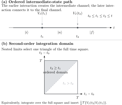
At second order, the interaction at $t_1$ acts before the interaction at $t_2$. Inserting completeness turns the operator product into a sum over intermediate states $\lvert n\rangle$. The ordered triangle has half the area of the full time square; the time-ordering operator provides an equivalent full-square representation.

Time-Ordering Notation

The second-order operator can also be written

$$\begin{aligned} U_I^{(2)}(t,t_0) ={}& \frac12 \left(-\frac{i}{\hbar}\right)^2 \\ &\times \int_{t_0}^{t}dt_2 \int_{t_0}^{t}dt_1\, \\ &\times \mathcal T \left\{ V_I(t_2)V_I(t_1) \right\}. \end{aligned}$$

For two bosonic operators in ordinary quantum mechanics, define $\mathcal O_{21}=\mathcal T\{V_I(t_2)V_I(t_1)\}$. Then

$$\mathcal O_{21} = \begin{cases} V_I(t_2)V_I(t_1),&t_2\gt t_1, \\ V_I(t_1)V_I(t_2),&t_1\gt t_2. \end{cases}$$

The factor $1/2!$ compensates for integrating both labeled orderings over the full square. The convention at $t_1=t_2$ does not affect ordinary integrals unless singular equal-time terms are present.

At order $r$, define the ordered integral

$$\begin{aligned} \mathcal K_r(t,t_0) ={}& \int_{t_0}^{t}dt_r \int_{t_0}^{t_r}dt_{r-1} \cdots \int_{t_0}^{t_2}dt_1\, \\ &\times V_I(t_r)V_I(t_{r-1}) \\ &\cdots V_I(t_1). \end{aligned}$$

Then

$$U_I^{(r)}(t,t_0) = \left(-\frac{i}{\hbar}\right)^r \mathcal K_r(t,t_0).$$

Equivalently, define the full-cube time-ordered integral

$$\begin{aligned} \mathcal Q_r(t,t_0) ={}& \int_{t_0}^{t}dt_r\cdots \int_{t_0}^{t}dt_1\, \\ &\times \mathcal T \left\{ V_I(t_r)\cdots V_I(t_1) \right\}. \end{aligned}$$

The same coefficient is

$$U_I^{(r)}(t,t_0) = \frac{1}{r!} \left(-\frac{i}{\hbar}\right)^r \mathcal Q_r(t,t_0).$$

The nested form is often best for explicit low-order calculations. The compact time-ordered form exposes the exponential structure and is the natural bridge to field theory.

A Sequential-Pulse Example

Consider three channels $\lvert i\rangle$, $\lvert n\rangle$, and $\lvert f\rangle$. Let the interaction-picture Hamiltonian contain

$$V_I(t) = g_1(t)\lvert n\rangle\langle i\rvert +g_2(t)\lvert f\rangle\langle n\rvert +\text{h.c.}$$

Assume $g_1$ acts in an early time window and $g_2$ in a later, nonoverlapping window. There is no direct $i\to f$ matrix element, so

$$\mathcal A_{fi}^{(1)}=0.$$

At second order, the only relevant ordered path is

$$\lvert i\rangle \xrightarrow{\,g_1(t_1)\,} \lvert n\rangle \xrightarrow{\,g_2(t_2)\,} \lvert f\rangle.$$

Its amplitude is

$$\begin{aligned} \mathcal A_{fi}^{(2)} ={}& \left(-\frac{i}{\hbar}\right)^2 \\ &\times \int dt_2\,g_2(t_2) \int^{t_2}dt_1\,g_1(t_1). \end{aligned}$$

Because every $g_1$ time precedes every $g_2$ time, the ordered integral factorizes:

$$\begin{aligned} \mathcal A_{fi}^{(2)} ={}& \left(-\frac{i}{\hbar}\right)^2 \\ &\times \left(\int dt_2\,g_2(t_2)\right) \\ &\times \left(\int dt_1\,g_1(t_1)\right). \end{aligned}$$

If the pulse order is reversed and the Hamiltonian contains no other path, this particular second-order amplitude vanishes: the operator that requires population in $\lvert n\rangle$ acts before $\lvert n\rangle$ has been created. Time ordering is therefore physical causal bookkeeping, not decorative notation.

Virtual Intermediate States

An intermediate state in the completeness sum need not be populated as an asymptotic or measured outcome. In an off-resonant two-step process, its contribution can remain transient and enter through an energy denominator after the time integrals are evaluated.

For a constant interaction switched on over $0\le t\le T$,

$$\begin{aligned} \mathcal A_{fi}^{(2)}(T) ={}& \left(-\frac{i}{\hbar}\right)^2 \sum_nV_{fn}V_{ni} \\ &\times \int_0^Tdt_2\,e^{i\omega_{fn}t_2} \\ &\times \int_0^{t_2}dt_1\,e^{i\omega_{ni}t_1}. \end{aligned}$$

For $\omega_{ni}\ne0$, the inner integral is

$$\int_0^{t_2}dt_1\,e^{i\omega_{ni}t_1} = \frac{e^{i\omega_{ni}t_2}-1}{i\omega_{ni}}.$$

The factor $1/\omega_{ni}$ is the finite-time ancestor of an intermediate-state energy denominator. Precise infinite-time denominators and their $i0$ prescriptions depend on switching, boundary conditions, and whether one is computing bound-state response or scattering. They should not be inserted by memory before the time protocol is specified.

If an intermediate detuning becomes small, the denominator is a warning rather than an enhancement formula to trust blindly. The near-resonant state may need to be included in a coupled model space and evolved nonperturbatively.

Selection Rules by Order

Suppose a symmetry makes

$$\langle f\rvert V_I(t)\lvert i\rangle=0.$$

Then the first-order amplitude vanishes. A second-order amplitude may still exist if there are intermediate states for which

$$\langle n\rvert V_I(t_1)\lvert i\rangle\ne0$$

and

$$\langle f\rvert V_I(t_2)\lvert n\rangle\ne0.$$

For example, if $V$ is odd under parity, one insertion changes parity. Two insertions have even overall parity, so states of the same parity can be connected at second order through opposite-parity intermediate states.

If $f\ne i$ and $\mathcal A_{fi}^{(1)}=0$, then

$$\mathcal A_{fi} = \lambda^2\mathcal A_{fi}^{(2)} +O(\lambda^3),$$

and the leading probability is

$$P_{i\to f} = \lambda^4 \lvert\mathcal A_{fi}^{(2)}\rvert^2 +O(\lambda^5).$$

Calling such a probability “second order” is ambiguous. It is second order in the amplitude and fourth order in the coupling at the probability level. State which convention is being used.

Probability Through the Next Order

For a previously empty final channel,

$$\mathcal A_{fi} = \lambda\mathcal A_{fi}^{(1)} +\lambda^2\mathcal A_{fi}^{(2)} +O(\lambda^3).$$

Squaring gives

$$\begin{aligned} P_{i\to f} ={}& \lambda^2 \lvert\mathcal A_{fi}^{(1)}\rvert^2 \\ &+2\lambda^3 \operatorname{Re} \left[ \mathcal A_{fi}^{(1)*} \mathcal A_{fi}^{(2)} \right] +O(\lambda^4). \end{aligned}$$

The second-order amplitude is needed for the cubic correction to a generic transition probability. To know the probability completely through $O(\lambda^4)$, one also needs the third-order amplitude because it interferes with the first-order term:

$$\begin{aligned} P_{i\to f}^{[4]} ={}& \lambda^4 \left\lvert\mathcal A_{fi}^{(2)}\right\rvert^2 \\ &+2\lambda^4 \operatorname{Re} \left[ \mathcal A_{fi}^{(1)*} \mathcal A_{fi}^{(3)} \right]. \end{aligned}$$

Computing “the probability to second order” therefore requires a declared counting convention.

Unitarity Order by Order

The exact $U_I$ is unitary. Insert

$$U_I=I+\lambda U_I^{(1)}+\lambda^2U_I^{(2)}+\cdots$$

into $U_I^\dagger U_I=I$. At first order,

$$U_I^{(1)}+U_I^{(1)\dagger}=0.$$

At second order,

$$U_I^{(2)} +U_I^{(2)\dagger} +U_I^{(1)\dagger}U_I^{(1)} = 0.$$

Taking an initial-state matrix element and inserting completeness gives

$$2\operatorname{Re}\mathcal A_{ii}^{(2)} + \sum_f \left\lvert\mathcal A_{fi}^{(1)}\right\rvert^2 = 0.$$

This identity connects the real part of the second-order forward amplitude with the total first-order probability flowing into all channels. It is the finite-dimensional ancestor of optical-theorem logic.

The survival probability becomes

$$\begin{aligned} P_{i\to i} ={}&1 -\lambda^2 \sum_{f\ne i} \left\lvert\mathcal A_{fi}^{(1)}\right\rvert^2 \\ &+O(\lambda^3). \end{aligned}$$

Thus probability loss from the initial channel appears at the same order as probability gained by the other channels. Keeping only the first-order survival amplitude misses this normalization mechanism.

Convergence and Truncation

For a bounded interaction on a finite interval, define

$$\eta(t) = \frac{\lvert\lambda\rvert}{\hbar} \int_{t_0}^{t}dt'\, \lVert V_I(t')\rVert.$$

The volume of the ordered $r$-simplex gives the bound

$$\left\lVert \lambda^rU_I^{(r)} \right\rVert \le \frac{\eta(t)^r}{r!}.$$

Consequently, the operator-norm remainder after order $N$ obeys a conservative estimate of the form

$$\lVert R_{N+1}\rVert \le e^{\eta} \frac{\eta^{N+1}}{(N+1)!}.$$

This estimate establishes convergence for bounded integrable interactions, but it ignores oscillatory cancellation and is often much less sharp than channel-specific phase estimates. For unbounded operators, domain and relative-boundedness questions require additional analysis; the formal Dyson series is not automatically an operator-norm theorem.

Even when the series converges for every finite time, a low-order truncation can become inaccurate when $\eta$ or a resonant channel amplitude is not small. Convergence of the infinite series and usefulness of the first few terms are different questions.

Finite-order unitarity

A truncated Dyson polynomial is not exactly unitary, although it satisfies unitarity identities through its retained order when used consistently. If exact finite-order unitarity is operationally important, a Magnus Expansion exponentiates anti-Hermitian generators and may be a better organization. Magnus has its own convergence and commutator costs; it is not universally superior.

Diagrammatic Intuition and the QFT Bridge

The inserted completeness relation suggests a diagrammatic reading:

• each interaction insertion is a vertex labeled by its time and operator;
• each segment between vertices carries an intermediate state and its phase;
• one sums over all allowed intermediate states;
• one integrates over all ordered vertex times;
• symmetry can remove entire paths by setting a vertex matrix element to zero.

This is useful bookkeeping, but it is not yet a Feynman diagram expansion. In quantum field theory, fields contain creation and annihilation operators, Wick’s theorem reorganizes time-ordered products into contractions, propagators encode field correlations, and diagram symmetry factors must be tracked.

The exact bridge begins at From Evolution Operators to Time-Ordered Products and QFT Bridge: S-Matrix. The reusable idea is already present here: amplitudes are ordered sums over interaction histories, and probabilities require coherent interference among those histories before squaring.

A Reliable Workflow

1. Fix the interaction picture. State $H_0$, $V_I(t)$, $t_0$, and all coupling constants.
2. Specify initial and final channels. Include their normalization and whether the final set is discrete or continuous.
3. Choose the amplitude order. Draw or list every allowed chain of matrix elements before integrating.
4. Insert completeness in an adapted basis. Use energy, symmetry, or channel labels that expose zeros and phases.
5. Enforce time ordering. Use nested limits or the time-ordering operator, but do not mix conventions or double count.
6. Evaluate finite-time integrals before taking limits. Switching functions and detunings determine denominators and resonance widths.
7. Convert amplitude order to probability order explicitly. Include interference with adjacent orders when required.
8. Check unitarity and depletion. Forward amplitudes and transition sums must satisfy the perturbative normalization identities.
9. Reorganize near small denominators or secular growth. Enlarge the model space, resum, or choose a better frame.
10. State what the diagrams mean. In ordinary quantum mechanics they are ordered state paths unless a field-theoretic contraction expansion has actually been introduced.

Common Mistakes

• Reversing operator order. In $V_I(t_2)V_I(t_1)$ with $t_2\ge t_1$, the rightmost $V_I(t_1)$ acts first.
• Integrating the full square without $1/2!$ and time ordering. This double counts labeled orderings.
• Forgetting the intermediate-state sum. A second-order transition can proceed through every state allowed by both matrix elements, including continuum channels.
• Treating an intermediate state as necessarily occupied. Off-resonant virtual channels need not appear as measured final outcomes.
• Inserting energy denominators before specifying switching. Finite-time integrals determine denominators, resonance factors, and boundary prescriptions.
• Calling a second-order amplitude an $O(\lambda^2)$ probability. If first order vanishes, its squared probability is usually $O(\lambda^4)$.
• Computing $\lvert\mathcal A^{(2)}\rvert^2$ and calling it the complete fourth-order probability. Interference between first- and third-order amplitudes also contributes.
• Checking normalization with mismatched orders. Survival and transition probabilities must be expanded consistently.
• Assuming a small denominator guarantees a large accurate answer. It often signals that fixed-order perturbation theory has chosen the wrong model space.
• Treating a truncated Dyson series as exactly unitary. Unitarity holds order by order only when all terms of the required order are retained.

Exercises

Show the two second-order forms agree

Prove that the nested second-order integral equals the full-square time-ordered expression with a factor $1/2!$.

Solution

Split the square $[t_0,t]^2$ into the two triangles $t_2\ge t_1$ and $t_1\ge t_2$. Then

$$\begin{aligned} &\frac12 \int_{t_0}^{t}dt_2 \int_{t_0}^{t}dt_1\, \mathcal T\{V_I(t_2)V_I(t_1)\} \\ ={}& \frac12 \int_{t_2\ge t_1}dt_2dt_1\, V_I(t_2)V_I(t_1) \\ &+ \frac12 \int_{t_1\ge t_2}dt_2dt_1\, V_I(t_1)V_I(t_2). \end{aligned}$$

Relabel $t_1\leftrightarrow t_2$ in the second triangle. It becomes identical to the first, so the factor $1/2$ cancels the two equal contributions:

$$\int_{t_0}^{t}dt_2 \int_{t_0}^{t_2}dt_1\, V_I(t_2)V_I(t_1).$$

Insert the intermediate states

Starting from $\langle f\rvert V_I(t_2)V_I(t_1)\lvert i\rangle$, derive the intermediate-state sum and state what changes if part of the spectrum is continuous.

Solution

Insert a complete discrete basis:

$$I=\sum_n\lvert n\rangle\langle n\rvert.$$

Then

$$\begin{aligned} \langle f\rvert V_I(t_2)V_I(t_1)\lvert i\rangle = \sum_n {}&\langle f\rvert V_I(t_2)\lvert n\rangle \\ &\times \langle n\rvert V_I(t_1)\lvert i\rangle. \end{aligned}$$

For a mixed discrete-continuum spectrum, completeness has the schematic form

$$I = \sum_{n\in\mathrm{disc}} \lvert n\rangle\langle n\rvert + \int dE\, \lvert E\rangle\langle E\rvert,$$

with normalization-dependent measures and channel labels included as needed. The intermediate sum then contains both a sum and an integral.

Reverse the sequential pulses

In the three-channel example, suppose the $g_2$ pulse is entirely earlier than the $g_1$ pulse. Show why the displayed path gives zero second-order amplitude.

Solution

The ordered amplitude contains

$$\int dt_2\,g_2(t_2) \int^{t_2}dt_1\,g_1(t_1).$$

Whenever $g_2(t_2)$ is nonzero, every time at which $g_1$ is nonzero lies later than $t_2$. The inner domain requires $t_1\le t_2$, so it contains no support of $g_1$ and vanishes.

This conclusion concerns the specific directed couplings displayed. Hermitian-conjugate terms or additional channels can create other ordered paths and must be examined separately.

Determine the leading probability order

An odd-parity perturbation connects an even initial state to an even final state only through odd-parity intermediate states. What are the leading amplitude and probability orders?

Solution

One odd operator changes parity, so

$$\mathcal A_{fi}^{(1)}=0$$

for even $i$ and even $f$. Two odd insertions have even overall parity and may connect through an odd intermediate state:

$$\mathcal A_{fi} = \lambda^2\mathcal A_{fi}^{(2)} +O(\lambda^3).$$

The leading probability is therefore

$$P_{i\to f} = \lambda^4 \left\lvert\mathcal A_{fi}^{(2)}\right\rvert^2 +O(\lambda^5),$$

unless another symmetry also removes the second-order paths.

Derive the unitarity identity

Expand $U_I^\dagger U_I=I$ through second order and derive the relation between the forward amplitude and the sum of first-order transition probabilities.

Solution

Write

$$U_I=I+\lambda U_1+\lambda^2U_2+O(\lambda^3).$$

Multiplication gives

$$\begin{aligned} U_I^\dagger U_I ={}&I +\lambda(U_1+U_1^\dagger) \\ &+\lambda^2(U_2+U_2^\dagger) \\ &+\lambda^2U_1^\dagger U_1 +O(\lambda^3). \end{aligned}$$

The second-order coefficient must vanish. Taking its expectation value in $\lvert i\rangle$ gives

$$2\operatorname{Re}\langle i\rvert U_2\lvert i\rangle + \langle i\rvert U_1^\dagger U_1\lvert i\rangle = 0.$$

Insert completeness into the last term:

$$\langle i\rvert U_1^\dagger U_1\lvert i\rangle = \sum_f \left\lvert\langle f\rvert U_1\lvert i\rangle\right\rvert^2.$$

Identifying the amplitude coefficients yields

$$2\operatorname{Re}\mathcal A_{ii}^{(2)} + \sum_f\left\lvert\mathcal A_{fi}^{(1)}\right\rvert^2 = 0.$$

Bound the ordered integral

Assume $\lVert V_I(t)\rVert\le V_{\max}$ for an interval of duration $T$. Bound the norm of the $r$th Dyson contribution including its coupling factor.

Solution

Submultiplicativity gives

$$\left\lVert V_I(t_r)\cdots V_I(t_1) \right\rVert \le V_{\max}^r.$$

The ordered integration region has volume

$$\frac{T^r}{r!}.$$

Therefore

$$\left\lVert \lambda^rU_I^{(r)} \right\rVert \le \frac{1}{r!} \left( \frac{\lvert\lambda\rvert V_{\max}T}{\hbar} \right)^r.$$

This bound is sufficient but often pessimistic because it discards phase cancellation and detailed matrix-element structure.

Cross-Links

• Time-Dependent Perturbation Theory and Transitions
• Interaction Picture for Perturbation Theory
• Dyson Expansion as Formal Evolution
• First-Order Transition Probability
• Fermi’s Golden Rule
• Selection Rules in Transition Rates
• Magnus Expansion
• From Evolution Operators to Time-Ordered Products
• QFT Bridge: S-Matrix
• Optical Theorem

References

• F. J. Dyson, “The radiation theories of Tomonaga, Schwinger, and Feynman,” Physical Review 75, 486–502, 1949.
• P. A. M. Dirac, The Principles of Quantum Mechanics, 4th ed., Oxford University Press, 1958.
• C. Cohen-Tannoudji, B. Diu, and F. Laloë, Quantum Mechanics, Vol. 2, Wiley, 1977.
• J. J. Sakurai and J. Napolitano, Modern Quantum Mechanics, 3rd ed., Cambridge University Press, 2020.
• S. Weinberg, The Quantum Theory of Fields, Vol. 1, Cambridge University Press, 1995.
• M. E. Peskin and D. V. Schroeder, An Introduction to Quantum Field Theory, Addison-Wesley, 1995.