Density of States in Transition Rates

In a transition rate, the density of states is the measure of how many distinct final states are available near the energy selected by the drive or interaction. It converts a probability for one normalized final state into a rate summed over a continuum. The result is trustworthy only when the state normalization, channel labels, degeneracy factors, and energy-shell Jacobian are all compatible with the matrix element.

This page owns that transition-rate bookkeeping. The elementary box-counting derivation lives in Density of States: First Encounter. The resolvent identity, local density of states, and spectral broadening live in Green Functions and Density of States. Compact state-counting formulas live in the Density of States formula card.

From a Final-State Sum to a Rate

Let $\lvert i\rangle$ be the prepared state and let $\lvert\alpha\rangle$ label exact final states with energies $E_\alpha$. A standard golden-rule expression is

$$\Gamma_i = \frac{2\pi}{\hbar} \sum_\alpha \lvert W_{\alpha i}\rvert^2 \delta(E_\alpha-E_*),$$

where

$$W_{\alpha i} = \langle\alpha\rvert W\lvert i\rangle.$$

The selected energy $E_*$ depends on the process. For a static perturbation,

$$E_*=E_i.$$

For absorption from a monochromatic drive,

$$E_*=E_i+\hbar\omega,$$

while stimulated emission selects $E_i-\hbar\omega$. The delta function is the long-time energy-selection limit; at finite time it is replaced by a kernel of width of order $\hbar/T$.

The exact density of final states is the distribution

$$\rho(E) = \sum_\alpha \delta(E-E_\alpha).$$

It has units of inverse energy when it counts a dimensionless number of states. A density per volume has units

$$[\rho/\mathcal V] = (\text{energy}\times\text{volume})^{-1}.$$

Density of states is not an occupation probability. It says what states exist, not which of them are populated.

The Weighted Density Is the Physical Object

The rate does not usually depend on $\rho(E)$ alone. Define the matrix-element-weighted density

$$\mathcal S_i(E) \equiv \sum_\alpha \lvert W_{\alpha i}\rvert^2 \delta(E-E_\alpha).$$

Then

$$\Gamma_i = \frac{2\pi}{\hbar} \mathcal S_i(E_*).$$

Only when the matrix element varies slowly among the states in the relevant energy window may one factorize

$$\mathcal S_i(E) \simeq \overline{ \lvert W(E)\rvert^2 } \rho(E).$$

This distinction prevents several common errors:

• a large density of states produces no transition if symmetry makes every relevant matrix element vanish;
• two channels with the same density of states can have very different rates;
• a threshold singularity in $\rho(E)$ can be softened or removed by a vanishing matrix element;
• pulling $\lvert W\rvert^2$ outside an integral is an approximation, not an identity.

The dimensions also check the formula. Since

$$[\mathcal S_i] = \text{energy},$$

the factor $2\pi/\hbar$ converts it to inverse time.

Channels and Continuum Coordinates

Suppose final states are organized into channels $c$ and continuous coordinates $\mathbf q$. A channel may encode spin, polarization, angular momentum, particle species, propagation direction, band index, or any other discrete label. Write the completeness measure schematically as

$$\sum_\alpha \longrightarrow \sum_c \int d\mu_c(\mathbf q).$$

The channel density of states is

$$\rho_c(E) = \int d\mu_c(\mathbf q)\, \delta\big(E-E_c(\mathbf q)\big),$$

and the total density is

$$\rho(E) = \sum_c\rho_c(E).$$

The rate is

$$\begin{aligned} \Gamma_i &= \frac{2\pi}{\hbar} \sum_c \int d\mu_c(\mathbf q)\, \\ &\quad\times \lvert W_{ci}(\mathbf q)\rvert^2 \delta\big(E_c(\mathbf q)-E_*\big). \end{aligned}$$

This form is safer than writing $\lvert W\rvert^2\rho$ prematurely because the integration measure and matrix element remain visibly paired.

The Energy-Shell Jacobian

For coordinates $\mathbf q\in\mathbb R^n$ with

$$d\mu_c(\mathbf q) = w_c(\mathbf q)d^nq,$$

the delta function restricts the integral to the constant-energy surface

$$\Sigma_{c,E} = \left\{ \mathbf q: E_c(\mathbf q)=E \right\}.$$

Away from critical points where $\nabla_{\mathbf q}E_c=0$, the coarea formula gives

$$\rho_c(E) = \int_{\Sigma_{c,E}} \frac{ w_c(\mathbf q)d\Sigma }{ \lVert\nabla_{\mathbf q}E_c\rVert }.$$

The factor

$$\frac{1}{ \lVert\nabla_{\mathbf q}E_c\rVert }$$

is the Jacobian that converts a coordinate-space shell thickness into an energy interval. Large constant-energy surfaces increase the density of states; a small energy gradient also increases it because many states fit into a narrow energy window.

At a band extremum, saddle point, flat band, or threshold, the gradient can vanish. The resulting density-of-states singularity may be physical, integrable, regularized by finite size or broadening, or modified by interactions. One should return to the original integral rather than substitute a formally divergent shell expression without analysis.

Box Normalization and Volume Cancellation

Continuum rates are often regulated by a periodic box of volume $\mathcal V=L^d$. The normalized plane waves are

$$\langle\mathbf x\vert\mathbf k\rangle_{\mathcal V} = \frac{1}{\sqrt{\mathcal V}} e^{i\mathbf k\cdot\mathbf x},$$

with

$$\mathbf k = \frac{2\pi}{L} \mathbf n, \qquad \mathbf n\in\mathbb Z^d.$$

The large-box sum becomes

$$\sum_{\mathbf k} \longrightarrow \frac{\mathcal V}{(2\pi)^d} \int d^dk.$$

For a localized initial state and localized interaction $W$, a typical box-normalized matrix element scales as

$$W_{\mathbf k i}^{(\mathcal V)} = \frac{1}{\sqrt{\mathcal V}} \mathcal M_i(\mathbf k),$$

where

$$\mathcal M_i(\mathbf k) = \int d^dx\, e^{-i\mathbf k\cdot\mathbf x} W(\mathbf x)\psi_i(\mathbf x)$$

in this convention. Consequently,

$$\left\lvert W_{\mathbf k i}^{(\mathcal V)} \right\rvert^2 = \frac{1}{\mathcal V} \lvert\mathcal M_i(\mathbf k)\rvert^2.$$

Substitution into the golden-rule sum gives

$$\begin{aligned} \Gamma_i &= \frac{2\pi}{\hbar} \frac{\mathcal V}{(2\pi)^d} \int d^dk\, \frac{ \lvert\mathcal M_i(\mathbf k)\rvert^2 }{\mathcal V} \\ &\qquad\times \delta\big(E(\mathbf k)-E_*\big) \\ &= \frac{2\pi}{\hbar} \int\frac{d^dk}{(2\pi)^d}\, \lvert\mathcal M_i(\mathbf k)\rvert^2 \delta\big(E(\mathbf k)-E_*\big). \end{aligned}$$

The artificial box volume cancels. If a purported rate for one localized emitter grows with the normalization volume, the continuum normalization has almost certainly been mixed inconsistently.

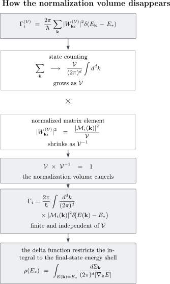
Box normalization makes the number of continuum states grow as $\mathcal V$, while each squared matrix element into a plane-wave state scales as $\mathcal V^{-1}$. Their product has a finite continuum limit. The cancellation must occur before interpreting the result as a physical rate.

Momentum Delta Normalization

One may bypass the box by choosing

$$\langle\mathbf x\vert\mathbf k\rangle = e^{i\mathbf k\cdot\mathbf x},$$

so that

$$\langle\mathbf k\vert\mathbf k'\rangle = (2\pi)^d \delta^{(d)}(\mathbf k-\mathbf k')$$

and

$$I = \int\frac{d^dk}{(2\pi)^d} \lvert\mathbf k\rangle \langle\mathbf k\rvert.$$

The continuum rate then has the volume-free form obtained above. Other conventions place factors of $(2\pi)^{d/2}$ in the wavefunction and use $\delta^{(d)}(\mathbf k-\mathbf k')$ without the prefactor. Either convention is valid if completeness, matrix elements, and density-of-states measures are transformed together.

Energy-Normalized States

Sometimes the density-of-states Jacobian is absorbed into the state normalization. Let $q$ be a one-dimensional continuum coordinate within channel $c$, with

$$\langle q,c\vert q',c'\rangle = \delta_{cc'}\delta(q-q').$$

Assume $E_c(q)$ is monotonic on that branch. Define

$$\lvert E,c\rangle = \frac{ \lvert q(E),c\rangle }{ \sqrt{ \left\lvert dE_c/dq\right\rvert } }.$$

Then

$$\langle E,c\vert E',c'\rangle = \delta_{cc'}\delta(E-E')$$

and

$$I_{\mathrm{cont}} = \sum_c \int dE\, \lvert E,c\rangle \langle E,c\rvert.$$

In this convention, the golden-rule rate is

$$\Gamma_i = \frac{2\pi}{\hbar} \sum_c \left\lvert \langle E_*,c\rvert W\lvert i\rangle \right\rvert^2.$$

No explicit $\rho(E_*)$ appears because the Jacobian is already inside $\lvert E,c\rangle$. The energy-normalized matrix element has different units from a box-normalized matrix element. Inserting an additional density of states would double count the same Jacobian.

If a given energy has several roots $q_j(E)$, each monotonic branch must be a separate channel or root label. In one dimension, for example, right- and left-moving states at the same energy account for the familiar factor of two unless the physical boundary condition selects only one direction.

Normalization Dictionary

Convention	Inner product	Completeness measure	Where the density factor lives
Finite box	$\delta_{\mathbf k\mathbf k'}$	$\sum_{\mathbf k}$	in the increasing number of discrete states
Momentum delta	$(2\pi)^d\delta^{(d)}(\mathbf k-\mathbf k')$	$\int d^dk/(2\pi)^d$	in the momentum measure and energy-shell Jacobian
Energy delta	$\delta_{cc'}\delta(E-E')$	$\sum_c\int dE$	absorbed into the definition of $\lvert E,c\rangle$

These are different coordinate descriptions of the same continuum. A calculation may change convention, but it must transform the states, completeness relation, and matrix element as a single package.

Free-Particle Examples in One, Two, and Three Dimensions

For a spinless nonrelativistic particle with threshold energy $E_{\mathrm{th}}$, define

$$\varepsilon \equiv E-E_{\mathrm{th}}, \qquad \varepsilon\gt0,$$

and dispersion

$$\varepsilon = \frac{\hbar^2k^2}{2m}.$$

Per box volume $\mathcal V_d$, the density of states in $d$ spatial dimensions is

$$\frac{\rho_d(\varepsilon)}{\mathcal V_d} = g_{\mathrm{int}} \frac{S_{d-1}}{(2\pi)^d} \frac{m}{\hbar^2} \left( \frac{\sqrt{2m\varepsilon}}{\hbar} \right)^{d-2},$$

where $g_{\mathrm{int}}$ counts included internal degeneracies and

$$S_{d-1} = \frac{2\pi^{d/2}}{ \Gamma(d/2) }$$

is the area of the unit sphere in $d$ dimensions. A factor $\Theta(\varepsilon)$ is understood.

The three most common cases are

$$\begin{array}{c|c} d & \rho_d(\varepsilon)/\mathcal V_d \\ \hline 1 & \displaystyle \frac{g_{\mathrm{int}}}{\pi\hbar} \sqrt{\frac{m}{2\varepsilon}} \\[0.9em] 2 & \displaystyle \frac{g_{\mathrm{int}}m}{2\pi\hbar^2} \\[0.9em] 3 & \displaystyle \frac{g_{\mathrm{int}}}{4\pi^2} \left( \frac{2m}{\hbar^2} \right)^{3/2} \sqrt{\varepsilon} \end{array}$$

Thus

$$\rho_d(\varepsilon) \propto \varepsilon^{d/2-1}.$$

• In one dimension the state density diverges as $\varepsilon^{-1/2}$ at threshold.
• In two dimensions it approaches a constant step.
• In three dimensions it vanishes as $\sqrt{\varepsilon}$.

These are density-of-states statements, not complete rate laws. The matrix element, channel boundary conditions, and any incident-flux factor can introduce additional powers of momentum.

Worked Energy-Shell Integral in Three Dimensions

Consider the volume-independent continuum expression

$$\begin{aligned} \Gamma_i &= \frac{2\pi}{\hbar} \int\frac{d^3k}{(2\pi)^3}\, \\ &\quad\times \lvert\mathcal M_i(\mathbf k)\rvert^2 \delta\left( \frac{\hbar^2k^2}{2m}-\varepsilon_* \right). \end{aligned}$$

Let

$$k_* = \frac{\sqrt{2m\varepsilon_*}}{\hbar}.$$

For $k\ge0$,

$$\delta\left( \frac{\hbar^2k^2}{2m}-\varepsilon_* \right) = \frac{m}{\hbar^2k_*} \delta(k-k_*).$$

Using $d^3k=k^2dk\,d\Omega_{\mathbf k}$ gives

$$\Gamma_i = \frac{2\pi}{\hbar} \frac{mk_*}{(2\pi)^3\hbar^2} \int d\Omega_{\mathbf k}\, \left\lvert \mathcal M_i(k_*,\Omega_{\mathbf k}) \right\rvert^2.$$

If the on-shell matrix element is isotropic,

$$\Gamma_i = \frac{2\pi}{\hbar} \lvert\mathcal M_i(k_*)\rvert^2 \frac{mk_*}{2\pi^2\hbar^2}.$$

The last factor is precisely the spinless three-dimensional density of states per volume in the momentum-delta convention appropriate to $\mathcal M_i$.

Threshold Scaling and Selection Rules

If the on-shell matrix element approaches a nonzero constant, the free-particle threshold scaling follows the density of states:

$$\Gamma(\varepsilon) \propto \varepsilon^{d/2-1}.$$

But angular momentum and symmetry often force the matrix element to vanish. If a partial-wave amplitude behaves as

$$\mathcal M_\ell(k) \propto k^\ell,$$

then in three dimensions

$$\Gamma_\ell \propto k^{2\ell+1} \propto \varepsilon^{\ell+1/2},$$

before long-range forces or other threshold effects are included. The density of states supplies only one part of the threshold law.

Selection Rules in Transition Rates explains how symmetry determines the zeros and allowed tensor structure of the matrix element.

Finite Time and the Continuum Window

A finite observation time $T$ resolves an energy window of order

$$\Delta E_T \sim \frac{\hbar}{T}.$$

Let $\delta E_{\mathrm{level}}$ be the typical spacing of final levels in a large but finite box. A smooth continuum approximation requires many levels inside the finite-time window:

$$\delta E_{\mathrm{level}} \ll \frac{\hbar}{T}.$$

Since

$$\delta E_{\mathrm{level}} \sim \frac{1}{\rho(E_*)},$$

the number of sampled levels is approximately

$$N_{\mathrm{win}} \sim \rho(E_*) \frac{\hbar}{T}.$$

One wants

$$N_{\mathrm{win}} \gg 1.$$

At the same time, the weighted density should vary little across that window. If $E_{\mathrm{var}}$ is its characteristic variation scale, require

$$\frac{\hbar}{T} \ll E_{\mathrm{var}}.$$

Together,

$$\delta E_{\mathrm{level}} \ll \frac{\hbar}{T} \ll E_{\mathrm{var}}.$$

The rate description also requires weak depletion,

$$\Gamma_iT \ll 1,$$

unless the exponential decay or master-equation resummation is performed. These inequalities define a time window; a continuum rate is not an exact all-time law for a finite closed system.

Multiple Channels and Degeneracy Factors

A reliable channel sum states what is included in $c$ and in $\rho_c$:

$$\Gamma_i = \sum_c\Gamma_{i\to c}.$$

Typical discrete factors include

• spin or helicity of the final particles;
• photon polarization;
• valleys, bands, subbands, or transverse modes;
• magnetic quantum numbers;
• right- and left-moving branches;
• particle species and reaction channels.

Initial-state quantum numbers are usually averaged only when the preparation is an incoherent mixture or the experiment does not resolve them. Final-state quantum numbers are summed when the measurement is inclusive over them. Identical final particles may require a symmetry factor rather than a naive label sum.

A degeneracy factor must appear exactly once. If $g_{\mathrm{int}}$ is already included in $\rho(E)$, summing the same internal states again in $\sum_c$ double counts them.

Bridge to Lorentz-Invariant Phase Space

In nonrelativistic many-particle problems, each final momentum contributes a measure such as

$$\frac{\mathcal V\,d^3p}{(2\pi\hbar)^3},$$

and conservation delta functions reduce the number of independent integrations. Relativistic QFT packages the corresponding final-state density into Lorentz-invariant phase space.

In natural units $\hbar=c=1$,

$$\begin{aligned} d\Phi_n(P) &= (2\pi)^4 \delta^{(4)}\left( P-\sum_{r=1}^{n}p_r \right) \\ &\quad\times \prod_{r=1}^{n} \frac{d^3p_r}{ (2\pi)^3 2E_r }. \end{aligned}$$

For a one-particle initial state of energy $E_i$, a decay-rate element has the schematic form

$$d\Gamma = \frac{1}{2E_i} \frac{1}{S} \overline{ \lvert\mathcal M\rvert^2 } d\Phi_n,$$

where $S$ accounts for identical-particle overcounting and the bar denotes any required spin sums or averages. Cross sections include an additional incident-flux factor.

The analogy with the nonrelativistic golden rule is structural:

$$\begin{aligned} \text{rate} &= \text{matrix element squared} \\ &\quad\times \text{final-state measure} \\ &\quad\times \text{conservation constraints}. \end{aligned}$$

Relativistic normalization changes every factor, so one should not transplant a nonrelativistic density of states into a QFT formula. See Scattering: QFT Bridge Reference for the broader dictionary.

A Reliable Workflow

1. List complete final-state labels. Separate continuous coordinates from discrete channels.
2. Write the normalization and completeness relation. Do this before evaluating matrix elements.
3. Keep the weighted sum intact. Start from $\sum_\alpha\lvert W_{\alpha i}\rvert^2\delta(E_\alpha-E_*)$.
4. Convert sums to integrals. Include every factor of volume, $2\pi$, $\hbar$, and degeneracy.
5. Apply the delta-function Jacobian. Retain all roots and branches of the energy constraint.
6. Check regulator cancellation. A physical localized rate should not depend on an artificial box size.
7. Test the continuum time window. Require many levels in $\hbar/T$ and slow variation across that window.
8. State what is summed or averaged. Include initial mixtures, final inclusiveness, and identical-particle factors.
9. Check dimensions. The final $\Gamma$ must have units of inverse time.

Common Mistakes

• Treating density of states as occupation. Availability and population are different objects.
• Multiplying by $\rho(E)$ after using energy-normalized states. That double counts the Jacobian.
• Mixing box-normalized and delta-normalized matrix elements. Their dimensions and volume scaling differ.
• Dropping roots of the energy equation. In one dimension, $k$ and $-k$ are distinct unless a channel condition removes one.
• Counting a degeneracy twice. Decide whether it belongs in $g_{\mathrm{int}}$, the channel sum, or the matrix element basis.
• Pulling a rapidly varying matrix element off shell. The factorized form $\lvert W\rvert^2\rho$ can fail near thresholds and resonances.
• Using the shell Jacobian at a critical point without care. Return to the unreduced integral when $\nabla E=0$.
• Taking the continuum limit at arbitrarily late times. A finite closed spectrum eventually resolves levels and can show recurrences.
• Using state density as a scattering cross section. Cross sections also require incident flux and the correct asymptotic normalization.

Exercises

Weighted versus unweighted density

Two final channels have the same density of states $\rho(E_*)$. Their on-shell matrix elements are $W_{1i}=w$ and $W_{2i}=0$. Compute the total rate and explain why $2\rho(E_*)\lvert w\rvert^2$ is incorrect.

Solution

The channel sum gives

$$\begin{aligned} \Gamma_i &= \frac{2\pi}{\hbar} \rho(E_*) \left( \lvert w\rvert^2+0 \right) \\ &= \frac{2\pi}{\hbar} \rho(E_*)\lvert w\rvert^2. \end{aligned}$$

The second channel contributes states but no transition strength. Replacing both channel matrix elements by $w$ ignores the selection-rule zero. The physical object is the weighted density, not the unweighted count alone.

Cancel the box volume

In $d$ dimensions, suppose

$$W_{\mathbf k i}^{(\mathcal V)} = \mathcal V^{-1/2}\mathcal M_i(\mathbf k).$$

Show explicitly that the golden-rule rate is independent of $\mathcal V$ in the continuum limit.

Solution

Use

$$\sum_{\mathbf k} \longrightarrow \frac{\mathcal V}{(2\pi)^d} \int d^dk$$

and

$$\left\lvert W_{\mathbf k i}^{(\mathcal V)} \right\rvert^2 = \frac{1}{\mathcal V} \lvert\mathcal M_i(\mathbf k)\rvert^2.$$

Then

$$\begin{aligned} \Gamma_i &= \frac{2\pi}{\hbar} \frac{\mathcal V}{(2\pi)^d} \int d^dk\, \\ &\quad\times \frac{\lvert\mathcal M_i(\mathbf k)\rvert^2}{\mathcal V} \delta(E_{\mathbf k}-E_*) \\ &= \frac{2\pi}{\hbar} \int\frac{d^dk}{(2\pi)^d}\, \lvert\mathcal M_i(\mathbf k)\rvert^2 \delta(E_{\mathbf k}-E_*). \end{aligned}$$

The volume from state counting cancels the inverse volume from the squared normalized matrix element.

Derive the dimensional threshold powers

For $\varepsilon=\hbar^2k^2/(2m)$, derive the scaling of the free-particle density of states in $d$ dimensions and specialize to $d=1,2,3$.

Solution

The number of states in a shell is proportional to

$$k^{d-1}dk.$$

Since

$$\frac{d\varepsilon}{dk} = \frac{\hbar^2k}{m},$$

one has

$$\rho_d(\varepsilon) \propto \frac{k^{d-1}}{d\varepsilon/dk} \propto k^{d-2}.$$

Using $k\propto\sqrt\varepsilon$ gives

$$\rho_d(\varepsilon) \propto \varepsilon^{d/2-1}.$$

Therefore

$$\rho_1\propto\varepsilon^{-1/2}, \qquad \rho_2\propto\varepsilon^0, \qquad \rho_3\propto\varepsilon^{1/2}.$$

Verify energy normalization

Assume $\langle q\vert q'\rangle=\delta(q-q')$ and a monotonic dispersion $E(q)$. Verify that

$$\lvert E\rangle = \frac{\lvert q(E)\rangle}{ \sqrt{\lvert dE/dq\rvert} }$$

satisfies $\langle E\vert E'\rangle=\delta(E-E')$.

Solution

The coordinate delta function transforms as

$$\delta\big(q(E)-q(E')\big) = \left\lvert \frac{dE}{dq} \right\rvert \delta(E-E').$$

Therefore

$$\begin{aligned} \langle E\vert E'\rangle &= \frac{ \delta\big(q(E)-q(E')\big) }{ \sqrt{\lvert dE/dq\rvert_E} \sqrt{\lvert dE/dq\rvert_{E'}} } \\ &= \delta(E-E'). \end{aligned}$$

On the support of the delta function, the two Jacobians are equal. If the dispersion has several roots at the same energy, each branch needs a separate channel label.

Find a golden-rule time window

Near $E_*$, let the mean final-level spacing be $\delta E$, let the weighted density vary on scale $E_{\mathrm{var}}$, and let the predicted rate be $\Gamma$. State inequalities on $T$ for a continuum golden-rule calculation without substantial depletion.

Solution

Many levels must lie inside the finite-time energy window:

$$\delta E \ll \frac{\hbar}{T}.$$

The weighted density must be nearly constant across that window:

$$\frac{\hbar}{T} \ll E_{\mathrm{var}}.$$

Finally, first-order depletion must remain small:

$$\Gamma T \ll 1.$$

Thus a useful interval requires

$$\frac{\hbar}{E_{\mathrm{var}}} \ll T \ll \min\left( \frac{\hbar}{\delta E}, \frac{1}{\Gamma} \right),$$

up to numerical factors set by the precise window convention. If no such interval exists, a constant continuum rate is not controlled.

Identify QFT counting factors

For a decay into two identical spinless particles, list the ingredients beyond $\lvert\mathcal M\rvert^2$ that are required in a relativistic rate.

Solution

The rate requires

• the invariant one-particle measures $d^3p_r/[(2\pi)^3 2E_r]$;
• a four-momentum delta function enforcing total energy and momentum conservation;
• the initial normalization factor $1/(2E_i)$;
• a symmetry factor $1/2!$ for two identical final particles when phase space labels would otherwise count each physical state twice;
• any required sums or averages over unresolved quantum numbers.

For a cross section rather than a decay rate, an incident-flux factor is also required. All factors must use one consistent relativistic state-normalization convention.

Cross-Links

• Fermi’s Golden Rule
• Time-Dependent Perturbation Theory and Transitions
• Density of States: First Encounter
• Green Functions and Density of States
• Density of States Formula Card
• Plane Waves and Delta Normalization
• Normalization Conventions
• Delta Function
• Selection Rules in Transition Rates
• Transition Rates shows how density conventions enter spectroscopy rates, differential channels, and cross sections.
• Linear Response Preview
• Transition Rates in Light–Matter Interaction
• Scattering: QFT Bridge Reference

References

• E. Fermi, Nuclear Physics, University of Chicago Press, 1950.
• C. Cohen-Tannoudji, B. Diu, and F. Laloë, Quantum Mechanics, Wiley, 1977.
• J. J. Sakurai and J. Napolitano, Modern Quantum Mechanics, 3rd ed., Cambridge University Press, 2020.
• R. Shankar, Principles of Quantum Mechanics, 2nd ed., Springer, 1994.
• N. W. Ashcroft and N. D. Mermin, Solid State Physics, Holt, Rinehart and Winston, 1976.
• M. E. Peskin and D. V. Schroeder, An Introduction to Quantum Field Theory, Addison-Wesley, 1995.