Linear Response Preview

Linear response asks for the first change in an observable produced by a weak external source. It does not require one to solve the fully driven problem. Instead, it packages the same matrix elements and transition frequencies that appear in time-dependent perturbation theory into a susceptibility.

For a perturbation

$$H(t)=H_0-f(t)B,$$

the response of an observable $A$ is written

$$\begin{aligned} \delta\langle A(t)\rangle ={}& \int_{-\infty}^{\infty}dt'\, \chi_{AB}^R(t,t')f(t') \\ & +O(f^2). \end{aligned}$$

The superscript $R$ means retarded: a source applied at $t'$ cannot alter an earlier measurement at $t$. In elementary quantum mechanics, the susceptibility is a sum over transitions. Its poles locate allowed transition frequencies, its residues contain matrix elements and populations, and its absorptive part reproduces the net golden-rule power absorbed from a harmonic drive.

This page owns that transition-theory bridge. Green Functions and Response Preview is the canonical home for the introductory Green-function conventions, analyticity, and harmonic-oscillator response. The Kubo Formula owns the full many-body treatment of spatial response, transport currents, contact terms, conserved quantities, equilibrium ensembles, and orders of limits.

What Linear Response Computes

Introduce a dimensionless bookkeeping parameter $\lambda$ if the source amplitude itself is not a convenient expansion parameter:

$$H(t;\lambda) = H_0-\lambda f(t)B.$$

For an observable with no explicit source dependence,

$$\langle A(t)\rangle_\lambda = \langle A(t)\rangle_0 + \lambda\,\delta^{(1)}\langle A(t)\rangle + O(\lambda^2).$$

Linear response computes the coefficient of $\lambda$. The physical source is restored by setting $\lambda=1$ only after the order counting is clear.

Three nearby quantities begin at different perturbative orders:

Quantity	Leading source order	Why
transition amplitude to a different level	$O(f)$	one interaction insertion
change in a general expectation value	$O(f)$	interference between unperturbed and first-order states
transition probability or absorbed power	$O(f^2)$	modulus square or source times induced response

The linearity refers to the observable response, not to every physical consequence. A susceptibility is first order in the induced expectation value, while the cycle-averaged work done by the drive is second order in its amplitude.

The source and detector are different roles

The operator $B$ specifies how the source perturbs the system. The operator $A$ specifies what is measured. They need not coincide:

Source $f$	Coupled operator $B$	Possible detector $A$
electric field	electric dipole	dipole or current
magnetic field	magnetic moment	magnetization
force	position	position or momentum
scalar potential	density	density or current

The notation $\chi_{AB}$ is ordered: it means the response of $A$ to a source coupled through $B$. Exchanging $A$ and $B$ generally changes the answer.

The Working Response Formula

Let the reference state be described by $\rho_0$ and suppose initially that

$$[H_0,\rho_0]=0.$$

Operators evolved with $H_0$ obey

$$A_H(t) = e^{iH_0t/\hbar} A e^{-iH_0t/\hbar}.$$

For the sign convention $H_{\mathrm{pert}}=-fB$, first-order time-dependent perturbation theory gives

$$\begin{aligned} \chi_{AB}^R(t-t') ={}& \frac{i}{\hbar} \theta(t-t') \\ &\times \operatorname{Tr} \left( \rho_0[A_H(t),B_H(t')] \right). \end{aligned}$$

This is the elementary Kubo response formula. A convention with $H_{\mathrm{pert}}=+fB$ reverses its overall sign.

The step function expresses causality. The commutator expresses the difference between the two possible operator orders and is what turns a correlation function into a response function. The formula is also the functional derivative

$$\chi_{AB}^R(t,t') = \left. \frac{\delta\langle A(t)\rangle_f} {\delta f(t')} \right|_{f=0}.$$

The derivation and the relation to retarded Green functions are developed at Green Functions and Response Preview. Here the formula is used as a calculational reorganization of transition amplitudes.

If the reference state is not stationary

Without $[H_0,\rho_0]=0$, the kernel generally depends on both times separately:

$$\chi_{AB}^R(t,t') \ne \chi_{AB}^R(t-t').$$

A single-frequency susceptibility $\chi(\omega)$ is then insufficient. One may need a two-frequency kernel, a Wigner transform with average and relative times, or a Floquet response function for a periodically driven reference state. Ordinary equilibrium-looking formulas should not be imported into that setting without rederivation.

From Transition Amplitudes to a Susceptibility

Take a pure reference eigenstate,

$$H_0\lvert i\rangle = E_i\lvert i\rangle,$$

and define

$$\omega_{ni} = \frac{E_n-E_i}{\hbar}.$$

The first-order interaction-picture amplitude generated by $-f(t)B$ is

$$\begin{aligned} c_n^{(1)}(t) ={}& \frac{i}{\hbar} B_{ni} \\ &\times \int_{t_0}^{t}dt'\, f(t')e^{i\omega_{ni}t'}, \\ & n\ne i. \end{aligned}$$

where $B_{ni}=\langle n\rvert B\lvert i\rangle$. The change in $\langle A(t)\rangle$ comes from interference between this first-order amplitude and the unperturbed amplitude. Collecting the term and its complex conjugate produces the commutator in $\chi_{AB}^R$.

This observation is the basic dictionary:

Transition-amplitude language	Response language
phase $e^{i\omega_{ni}t}$	pole at a transition frequency
coupling matrix element $B_{ni}$	source residue
measurement matrix element $A_{in}$	detector residue
initial-state weight	population factor
finite pulse Fourier transform	source spectrum sampled by $\chi$
sum over final states	spectral representation

Response theory does not discard the transition picture. It organizes all first-order transition pathways into the expectation value of the chosen detector.

Frequency-Domain Susceptibility

For a stationary reference state, set the earlier time to zero and use

$$\chi_{AB}^R(\omega) = \int_{-\infty}^{\infty}dt\, e^{i\omega t} \chi_{AB}^R(t).$$

The inverse convention is

$$\chi_{AB}^R(t) = \int_{-\infty}^{\infty} \frac{d\omega}{2\pi}\, e^{-i\omega t} \chi_{AB}^R(\omega).$$

Then convolution becomes multiplication:

$$\delta\langle A(\omega)\rangle = \chi_{AB}^R(\omega)f(\omega).$$

Diagonalize the stationary density operator within each degenerate energy subspace,

$$\rho_0 = \sum_n p_n\lvert n\rangle\langle n\rvert.$$

With

$$A_{nm}=\langle n\rvert A\lvert m\rangle, \qquad B_{mn}=\langle m\rvert B\lvert n\rangle,$$

the sum-over-states form is

$$\chi_{AB}^R(\omega) = \sum_{n,m} \frac{ (p_m-p_n)A_{nm}B_{mn} }{ \hbar\omega+E_n-E_m+i0^+ }.$$

The infinitesimal $i0^+$ records retarded support. It is a boundary prescription, not a physical decay rate.

What the spectral formula says

Each term contains four pieces:

1. Location: $E_m-E_n$ fixes the transition frequency.
2. Excitation strength: $B_{mn}$ says whether the source can couple the states.
3. Detection strength: $A_{nm}$ says whether the chosen observable sees the induced coherence.
4. Population contrast: $p_n-p_m$ distinguishes absorption from stimulated emission.

For self-response, take $A=B=B^\dagger$ and write

$$\chi_{BB}^R(\omega) = \chi_{BB}'(\omega) + i\chi_{BB}''(\omega).$$

Using

$$\frac{1}{x+i0^+} = \operatorname{PV}\frac{1}{x} - i\pi\delta(x),$$

the absorptive part is

$$\begin{aligned} \chi_{BB}''(\omega) ={}& \pi \sum_{n,m} (p_n-p_m) \\ &\times \lvert B_{mn}\rvert^2 \\ &\times \delta\!\left( \hbar\omega-E_m+E_n \right). \end{aligned}$$

Equivalently, for $\omega_{mn}=(E_m-E_n)/\hbar$,

$$\begin{aligned} \chi_{BB}''(\omega) ={}& \frac{\pi}{\hbar} \sum_{n,m} (p_n-p_m) \\ &\times \lvert B_{mn}\rvert^2 \delta(\omega-\omega_{mn}). \end{aligned}$$

At positive frequency, only upward energy differences contribute. For a passive state whose populations do not increase with energy, $\chi_{BB}''(\omega)\ge0$ for $\omega\gt0$ in this convention.

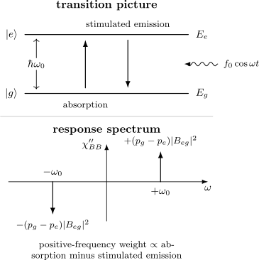
A single pair of levels appears in two languages. The harmonic source drives absorption and stimulated emission between the levels; the same matrix element produces opposite-sign peaks of $\chi_{BB}''(\omega)$ at $\pm\omega_0$. At positive frequency, the peak weight is proportional to the population difference $p_g-p_e$.

Dissipation and Golden-Rule Rates

Let the source be monochromatic,

$$f(t)=f_0\cos\omega t, \qquad \omega\gt0,$$

and take $B=B^\dagger$. For a pair with $E_m\gt E_n$, the rotating component of the source gives the golden-rule absorption rate per system initially in $\lvert n\rangle$,

$$\Gamma_{n\to m}^{\mathrm{abs}} = \frac{\pi f_0^2}{2\hbar^2} \lvert B_{mn}\rvert^2 \delta(\omega-\omega_{mn}).$$

The counter-rotating component gives stimulated emission from $m$ to $n$ at the same positive drive frequency,

$$\Gamma_{m\to n}^{\mathrm{stim}} = \frac{\pi f_0^2}{2\hbar^2} \lvert B_{nm}\rvert^2 \delta(\omega-\omega_{mn}).$$

Hermiticity gives $\lvert B_{nm}\rvert^2=\lvert B_{mn}\rvert^2$. The net energy gained by the system is therefore

$$\begin{aligned} \overline P(\omega) ={}& \hbar\omega \sum_{E_m\gt E_n} \left( p_n\Gamma_{n\to m}^{\mathrm{abs}} - p_m\Gamma_{m\to n}^{\mathrm{stim}} \right) \\ ={}& \frac{\omega f_0^2}{2} \chi_{BB}''(\omega). \end{aligned}$$

The same identity follows directly from work. Since $H_{\mathrm{pert}}=-fB$,

$$\frac{dW}{dt} = \left\langle \frac{\partial H}{\partial t} \right\rangle = -\dot f(t)\langle B(t)\rangle.$$

The induced response to $f_0\cos\omega t$ is

$$\begin{aligned} \delta\langle B(t)\rangle ={}& f_0 \chi_{BB}'(\omega)\cos\omega t \\ &+ f_0 \chi_{BB}''(\omega)\sin\omega t. \end{aligned}$$

Averaging $-\dot f\,\delta\langle B\rangle$ over one cycle leaves only the out-of-phase component and gives the same $\overline P$.

What is and is not included

• $\chi'$ describes the reactive, in-phase response and stores energy reversibly over a cycle.
• $\chi''$ describes the out-of-phase component and controls net work at order $f_0^2$.
• Stimulated emission appears because the classical source has both positive- and negative-frequency components.
• Spontaneous emission does not arise from a prescribed classical source. It requires coupling to quantized field modes or another environment.
• For a continuum of final states, the sum over $m$ becomes the weighted density-of-states integral developed in Density of States in Transition Rates.

The equality between $\chi''$ and net transition power is one of the cleanest bridges between time-dependent perturbation theory and response theory.

Finite Time, Delta Functions, and Linewidths

An isolated finite system observed for a finite duration does not literally produce an infinitely sharp spectral line. For a square observation window of duration $T$, the transition probability contains

$$\left| \int_0^Tdt\, e^{i\Delta\omega t} \right|^2 = T^2 \operatorname{sinc}^2 \left( \frac{\Delta\omega T}{2} \right).$$

The normalized finite-time delta sequence is

$$\delta_T(\Delta\omega) = \frac{T}{2\pi} \operatorname{sinc}^2 \left( \frac{\Delta\omega T}{2} \right),$$

with

$$\int_{-\infty}^{\infty} d(\Delta\omega)\, \delta_T(\Delta\omega) = 1.$$

Only after a suitable long-time or continuum limit may one replace $\delta_T$ by $\delta$. Three mechanisms that are often conflated must be kept separate:

Spectral width	Origin	Typical mathematical object
finite-time resolution	limited pulse or observation duration	sinc-like window function
lifetime broadening	irreversible decay or coupling to a bath	finite imaginary self-energy or damping rate
inhomogeneous broadening	distribution of transition frequencies	ensemble average over parameters

The retarded $i0^+$ chooses how a pole is approached. Replacing it by a finite $i\gamma$ asserts additional physics and must be justified by a decay model, a self-energy, or an explicitly phenomenological linewidth.

Worked Example: A Two-Level Susceptibility

Consider

$$H_0 = \frac{\hbar\omega_0}{2}\sigma_z, \qquad B=b\sigma_x, \qquad \omega_0\gt0.$$

Let $\lvert g\rangle$ be the ground state. Since

$$\lvert\langle e\rvert B\lvert g\rangle\rvert^2 = b^2,$$

the time-domain self-response is

$$\chi_{BB}^R(t) = \frac{2b^2}{\hbar} \theta(t) \sin\omega_0t.$$

Its frequency-domain form is

$$\begin{aligned} \chi_{BB}^R(\omega) ={}& \frac{b^2}{ \hbar(\omega+\omega_0+i0^+) } \\ &- \frac{b^2}{ \hbar(\omega-\omega_0+i0^+) }. \end{aligned}$$

The positive-frequency absorptive part is

$$\chi_{BB}''(\omega) = \frac{\pi b^2}{\hbar} \delta(\omega-\omega_0), \qquad \omega\gt0.$$

For $f(t)=f_0\cos\omega t$, the golden-rule excitation rate is

$$\Gamma_{g\to e} = \frac{\pi f_0^2b^2}{2\hbar^2} \delta(\omega-\omega_0).$$

Multiplying by the absorbed quantum $\hbar\omega$ gives

$$\hbar\omega\Gamma_{g\to e} = \frac{\omega f_0^2}{2} \chi_{BB}''(\omega),$$

as required.

Static check

At zero frequency,

$$\chi_{BB}^R(0) = \frac{2b^2}{\hbar\omega_0}.$$

This can be checked without response theory. The exact ground-state energy of

$$H = \frac{\hbar\omega_0}{2}\sigma_z - fb\sigma_x$$

is

$$E_g(f) = -\sqrt{ \left(\frac{\hbar\omega_0}{2}\right)^2 + f^2b^2 }.$$

The Hellmann–Feynman relation gives

$$\langle B\rangle_f = -\frac{dE_g}{df} = \frac{fb^2}{ \sqrt{(\hbar\omega_0/2)^2+f^2b^2} }.$$

Therefore

$$\left. \frac{d\langle B\rangle_f}{df} \right|_{f=0} = \frac{2b^2}{\hbar\omega_0},$$

which agrees with $\chi_{BB}^R(0)$. This is a useful normalization and sign check.

Population inversion

For a stationary mixture with ground- and excited-state populations $p_g$ and $p_e$,

$$\begin{aligned} \chi_{BB}''(\omega) ={}& \frac{\pi b^2}{\hbar} (p_g-p_e) \\ &\times \delta(\omega-\omega_0), \qquad \omega\gt0. \end{aligned}$$

If $p_e\gt p_g$, the absorptive part is negative and the probe gains energy. This is small-signal gain about an inverted reference state, not a violation of energy conservation: energy was supplied when the inversion was prepared.

Static Response and Ordinary Perturbation Theory

For a nondegenerate ground state and Hermitian $B$, the zero-frequency susceptibility is

$$\chi_{BB}^R(0) = 2 \sum_{n\ne0} \frac{ \lvert\langle n\rvert B\lvert0\rangle\rvert^2 }{ E_n-E_0 }.$$

This is exactly the result obtained from the first-order correction to the ground state under the static perturbation $-fB$. Static perturbation theory and zero-frequency response are therefore two views of the same derivative, provided the limits are regular.

The qualification matters. Near degeneracy, in a continuum, or in a thermodynamic limit, the operations

$$\begin{gathered} \omega\to0, \qquad \mathbf q\to0, \\ V\to\infty, \qquad \gamma\to0^+ \end{gathered}$$

need not commute. A finite few-level system hides many of the subtleties that dominate transport and collective response.

For the canonical state-correction machinery, see First-Order State Corrections.

Selection Rules in Response

The spectral numerator $A_{nm}B_{mn}$ separates excitation from detection:

• If symmetry forces $B_{mn}=0$, the source does not drive that transition at first order.
• If $B_{mn}\ne0$ but $A_{nm}=0$, the source can create the coherence but the chosen detector has no linear signal from that pathway.
• Several intermediate states can contribute with phases, so a cross-susceptibility need not be a sum of positive terms.
• For self-response with a Hermitian $B$, the spectral weights reduce to nonnegative matrix-element magnitudes multiplied by population differences.

Parity, angular momentum, exchange symmetry, and tensor rank constrain the same matrix elements here as in transition-rate calculations. The canonical discussion is Selection Rules in Transition Rates.

Validity and Breakdown

Linear response is a controlled first-order expansion only while the induced change remains small in the sense relevant to the observable and state.

For a pure initial eigenstate, a useful channel diagnostic is

$$\epsilon_{ni}(t) = \frac{1}{\hbar} \left| B_{ni} \int_{t_0}^{t}dt'\, f(t')e^{i\omega_{ni}t'} \right|.$$

One requires the relevant $\epsilon_{ni}$ and the total leaked probability to remain small. A small instantaneous source does not guarantee a small accumulated response near resonance.

Situation	Linear-response status	Better treatment when it fails
weak, off-resonant, finite-duration drive	usually controlled	higher perturbative orders if needed
resonant drive for a long time	secular growth can invalidate truncation	Rabi or rotating-frame dynamics
dense continuum with an intermediate-time window	rate description may emerge	golden rule with normalization audit
appreciable depletion or saturation	population change feeds back on response	master equation or nonperturbative drive
strong damping or structured environment	isolated susceptibility is incomplete	open-system response or self-energy methods
periodically driven reference state	one-frequency stationary response fails	Floquet response
collective transport	contact terms and orders of limits matter	full many-body Kubo formalism

The weak-drive Rabi Formula in the Weak-Drive Limit and the nonperturbative Rabi Oscillations: First Encounter show explicitly how resonant first-order growth gives way to bounded population oscillations.

Kubo Formula Preview and Boundary

The compact formula

$$\begin{aligned} \delta\langle A(t)\rangle ={}& \int dt'\, f(t') \\ &\times \frac{i}{\hbar} \theta(t-t') \\ &\times \langle[A_H(t),B_H(t')]\rangle_0. \end{aligned}$$

is the elementary core of Kubo response. The canonical Kubo Formula page develops the source-to-response derivation and the additional ingredients a mature many-body calculation must specify:

• whether the reference state is equilibrium, a generalized ensemble, or nonequilibrium;
• spatial arguments and momentum transfer, such as $\chi_{AB}(\mathbf q,\omega)$;
• extensive versus intensive normalization;
• current operators and any explicit source dependence of the measured observable;
• diamagnetic or other contact terms;
• conserved quantities and hydrodynamic singularities;
• the order of uniform, static, thermodynamic, and zero-damping limits;
• analytic continuation when starting from imaginary-time correlators.

Equilibrium also supplies relations between spontaneous fluctuations and dissipative response. Those additional assumptions and quantum thermal factors belong to the Fluctuation–Dissipation Relation. Linear response by itself does not imply thermal equilibrium.

Calculation Workflow

1. Fix the sign: write the perturbation explicitly as $-fB$ or $+fB$.
2. Name the detector: state which observable $A$ is measured.
3. Specify the reference state: give $\rho_0$ and check whether it is stationary.
4. Choose conventions: state the Fourier transform and the retarded prescription.
5. Evaluate matrix elements: apply symmetry before summing states.
6. Separate regimes: distinguish a finite pulse, a discrete spectrum, and a continuum rate limit.
7. Interpret both parts: identify reactive response from $\chi'$ and net work from $\chi''$.
8. Audit validity: estimate accumulated amplitudes, depletion, damping, and resonance time scales.
9. Cross-check: compare $\chi(0)$ with static perturbation theory or compare $\chi''$ with golden-rule power.

Common Mistakes

• Omitting the sign of the source coupling and then comparing susceptibilities across conventions.
• Treating $A$ and $B$ as interchangeable in a cross-susceptibility.
• Calling an ordinary, time-ordered, or symmetrized correlator a causal response function.
• Forgetting that an $O(f)$ induced observable can produce $O(f^2)$ absorbed power.
• Reading every pole as an allowed transition without checking source and detector matrix elements.
• Dropping the population difference and thereby losing stimulated emission.
• Interpreting $i0^+$ as a measured linewidth.
• Replacing a finite-time sinc profile by a delta function before a rate window exists.
• Using a stationary $\chi(\omega)$ for a nonstationary reference state.
• Assuming that a large resonant response remains in the linear regime merely because $f_0$ is small.
• Applying an equilibrium fluctuation–dissipation relation to a generic driven state.
• Taking static, uniform, thermodynamic, and zero-damping limits without specifying their order.

Exercises

1. Recover the commutator from transition amplitudes

For an initial eigenstate $\lvert i\rangle$ and perturbation $-f(t)B$, insert the first-order amplitudes into $\langle A(t)\rangle$. Show that the result can be written with the retarded commutator.

Solution

To first order, the interaction-picture state is

$$\lvert\psi_I(t)\rangle = \lvert i\rangle + \frac{i}{\hbar} \int_{t_0}^{t}dt'\, f(t')B_I(t')\lvert i\rangle.$$

The first-order change in the expectation value is the sum of the ket correction and its adjoint:

$$\begin{aligned} C_{AB}(t,t') &= \langle i\rvert A_I(t)B_I(t') \lvert i\rangle, \\ C_{BA}(t',t) &= \langle i\rvert B_I(t')A_I(t) \lvert i\rangle. \end{aligned}$$

In this notation,

$$\begin{aligned} \delta\langle A(t)\rangle ={}& \frac{i}{\hbar} \int_{t_0}^{t}dt'\, f(t') C_{AB}(t,t') \\ &- \frac{i}{\hbar} \int_{t_0}^{t}dt'\, f(t') C_{BA}(t',t). \end{aligned}$$

Combining the terms gives

$$\begin{aligned} \delta\langle A(t)\rangle ={}& \frac{i}{\hbar} \int_{t_0}^{t}dt'\, f(t') \\ &\times \langle i\rvert [A_I(t),B_I(t')] \lvert i\rangle. \end{aligned}$$

Extending the integral over all $t'$ inserts $\theta(t-t')$, which is the retarded response kernel.

2. Verify the two-level static response

Expand the exact ground-state expectation $\langle B\rangle_f$ for the two-level example through cubic order in $f$. Identify the linear susceptibility and the first nonlinear correction.

Solution

The exact result is

$$\langle B\rangle_f = \frac{fb^2}{ \sqrt{(\hbar\omega_0/2)^2+f^2b^2} }.$$

Factor out $\hbar\omega_0/2$ and expand $(1+x)^{-1/2}=1-x/2+O(x^2)$:

$$\begin{aligned} \langle B\rangle_f ={}& \frac{2b^2}{\hbar\omega_0}f \\ &- \frac{4b^4}{\hbar^3\omega_0^3}f^3 + O(f^5). \end{aligned}$$

Thus

$$\chi_{BB}^R(0) = \frac{2b^2}{\hbar\omega_0},$$

while the cubic term is the first nonlinear correction. There is no quadratic term because this model is invariant under simultaneously reversing $f$ and $\sigma_x$.

3. Check the power–rate identity

For one pair $E_m-E_n=\hbar\omega$, use the golden-rule absorption and stimulated-emission rates to derive its contribution to $\overline P=(\omega f_0^2/2)\chi_{BB}''$.

Solution

The population-weighted net rate is

$$\begin{aligned} &p_n\Gamma_{n\to m}^{\mathrm{abs}} - p_m\Gamma_{m\to n}^{\mathrm{stim}} \\ &\quad= \frac{\pi f_0^2}{2\hbar^2} (p_n-p_m) \\ &\qquad\times \lvert B_{mn}\rvert^2 \delta(\omega-\omega_{mn}). \end{aligned}$$

Multiplying by the energy $\hbar\omega$ gives

$$\begin{aligned} \overline P_{nm} ={}& \frac{\pi\omega f_0^2}{2\hbar} (p_n-p_m) \\ &\times \lvert B_{mn}\rvert^2 \delta(\omega-\omega_{mn}). \end{aligned}$$

The same pair contributes

$$\begin{aligned} \chi_{BB,nm}''(\omega) ={}& \frac{\pi}{\hbar} (p_n-p_m) \\ &\times \lvert B_{mn}\rvert^2 \delta(\omega-\omega_{mn}), \end{aligned}$$

so $\overline P_{nm}=(\omega f_0^2/2)\chi_{BB,nm}''$.

4. Normalize the finite-time line shape

Show that

$$\delta_T(x) = \frac{T}{2\pi} \operatorname{sinc}^2 \left(\frac{xT}{2}\right)$$

has unit integral. What sets its characteristic width?

Solution

Set $u=xT/2$, so $dx=2du/T$. Then

$$\begin{aligned} \int_{-\infty}^{\infty}dx\,\delta_T(x) &= \frac{1}{\pi} \int_{-\infty}^{\infty}du\, \left(\frac{\sin u}{u}\right)^2 \\ &=1, \end{aligned}$$

using the standard integral $\int_{-\infty}^{\infty}du\,(\sin u/u)^2=\pi$. The first zeros occur at $x=\pm2\pi/T$, so the width scales as $1/T$.

5. Diagnose gain from an inverted pair

For the two-level mixture, suppose $p_e=3/4$ and $p_g=1/4$. Determine the sign of $\chi_{BB}''(\omega_0)$ and of the cycle-averaged power delivered to the system.

Solution

The positive-frequency spectral weight is proportional to

$$p_g-p_e = -\frac12.$$

Therefore $\chi_{BB}''(\omega_0)$ is negative. Since

$$\overline P = \frac{\omega_0f_0^2}{2} \chi_{BB}''(\omega_0),$$

the power delivered to the system is also negative. The system transfers energy to the probe through net stimulated emission.

6. Decide whether a Lorentzian is justified

An isolated two-level system is driven for a finite square pulse. A calculation replaces $i0^+$ by $i\gamma$ and interprets $\gamma$ as the measured linewidth, but no decay process is specified. What is wrong, and what line shape follows from the stated setup?

Solution

The replacement introduces a finite lifetime or dephasing scale that is absent from the model. The retarded $i0^+$ fixes the boundary value of an ideal pole; it does not supply a physical linewidth.

For a finite square pulse, the transition probability has the sinc-squared profile

$$T^2 \operatorname{sinc}^2 \left( \frac{(\omega-\omega_0)T}{2} \right),$$

whose width is set by $1/T$. A Lorentzian requires additional exponential decay, a bath model, a self-energy, or an explicitly stated phenomenological assumption.

Cross-Links

• Time-Dependent Perturbation Theory and Transitions
• Interaction Picture for Perturbation Theory
• First-Order Transition Probability
• Harmonic Perturbations
• Fermi’s Golden Rule
• Density of States in Transition Rates
• Selection Rules in Transition Rates
• Transition Rates in Light–Matter Interaction
• Green Functions and Response Preview
• Spectral Representation of Green Functions
• Kubo Formula
• Fluctuation–Dissipation Relation

References

• R. Kubo, “Statistical-mechanical theory of irreversible processes. I: General theory and simple applications to magnetic and conduction problems,” Journal of the Physical Society of Japan 12, 570–586 (1957), doi:10.1143/JPSJ.12.570.
• H. B. Callen and T. A. Welton, “Irreversibility and generalized noise,” Physical Review 83, 34–40 (1951), doi:10.1103/PhysRev.83.34.
• R. Kubo, “The fluctuation-dissipation theorem,” Reports on Progress in Physics 29, 255–284 (1966), doi:10.1088/0034-4885/29/1/306.
• J. J. Sakurai and J. Napolitano, Modern Quantum Mechanics, 3rd ed., Cambridge University Press, 2020.
• G. D. Mahan, Many-Particle Physics, 3rd ed., Kluwer Academic/Plenum, 2000.
• A. L. Fetter and J. D. Walecka, Quantum Theory of Many-Particle Systems, Dover, 2003.