Sudden Approximation

The sudden approximation describes a Hamiltonian change completed so quickly that the quantum state has negligible time to evolve during the change. Immediately after an ideal sudden quench, the ket is therefore the same vector as immediately before it. What changes is the Hamiltonian, its eigenbasis, and the energy distribution assigned to that unchanged state.

This page is the canonical home for abrupt Hamiltonian changes as an approximation method. Quantum Quenches owns the subsequent many-body initial-value protocol, correlation fronts, entanglement growth, and return amplitudes. The exact framework for arbitrary time dependence lives in Time-Dependent Hamiltonians. Work Distributions owns the thermodynamic measurement protocol, while Squeezed States: First Encounter owns the general squeeze-operator formalism.

The Sudden Regime

Let a control parameter change from $\lambda_i$ to $\lambda_f$ over a quench interval

$$t_i\le t\le t_f, \qquad \tau_q\equiv t_f-t_i,$$

and let

$$H(t)=H\big(\lambda(t)\big).$$

The exact evolution across the interval is

$$\begin{aligned} U_q &\equiv U(t_f,t_i) \\ &= \mathcal T \exp\left[ -\frac{i}{\hbar} \int_{t_i}^{t_f}H(t)\,dt \right]. \end{aligned}$$

The sudden approximation is

$$U_q \simeq e^{i\phi_q}I$$

on the states or subspace relevant to the calculation. The scalar phase $\phi_q$ has no effect on probabilities. Thus the physical statement is not that the Hamiltonian changes by a small amount. The change $H_i\to H_f$ may be large. The statement is that the integrated nontrivial action accumulated during the short switching interval is small.

A common time-scale estimate is

$$\frac{\tau_q\Delta E_{\mathrm{char}}}{\hbar} \ll 1,$$

or equivalently

$$\tau_q \ll \frac{1}{\omega_{\mathrm{char}}}, \qquad \omega_{\mathrm{char}} = \frac{\Delta E_{\mathrm{char}}}{\hbar}.$$

The phrase “characteristic energy” must be tied to the prepared state and to the matrix elements activated by the protocol. It is not automatically the smallest gap, the largest eigenvalue of an unbounded Hamiltonian, or the final level spacing.

An Operator-Norm Criterion

For a bounded Hamiltonian on a finite-dimensional space or controlled subspace, separate an arbitrary scalar part:

$$H(t) = E_{\mathrm{ref}}(t)I + K(t).$$

Define the integrated action

$$\mathcal A_q \equiv \frac{1}{\hbar} \int_{t_i}^{t_f} \lVert K(t)\rVert\,dt.$$

The scalar term contributes

$$\Phi_q = \frac{1}{\hbar} \int_{t_i}^{t_f} E_{\mathrm{ref}}(t)\,dt.$$

Duhamel’s formula gives the useful bound

$$\left\lVert U_q-e^{-i\Phi_q}I \right\rVert \le \mathcal A_q.$$

Therefore

$$\mathcal A_q\ll1$$

is a sufficient suddenness condition on that space. Subtracting $E_{\mathrm{ref}}I$ matters: a large common energy offset generates only a global phase and should not make an otherwise sudden protocol appear inaccurate.

For an unbounded Hamiltonian, the full operator norm may be infinite. One then needs a state-specific estimate, an energy-restricted subspace, a quadratic-form argument, or a theorem adapted to the model. A useful first-order diagnostic for a fixed initial ket is

$$\epsilon_i \equiv \frac{1}{\hbar} \int_{t_i}^{t_f} \Delta_i H(t)\,dt,$$

where

$$\begin{aligned} \big(\Delta_iH(t)\big)^2 &= \langle\psi_i\rvert H^2(t)\lvert\psi_i\rangle \\ &\quad- \langle\psi_i\rvert H(t)\lvert\psi_i\rangle^2. \end{aligned}$$

If $\epsilon_i\ll1$, the state changes only weakly beyond an overall phase at leading order. This is a diagnostic, not a universal error theorem for every unbounded or many-body problem.

Ideal Instantaneous Quench

The idealized protocol is

$$H(t) = \begin{cases} H_i, & t\lt0,\\ H_f, & t\gt0. \end{cases}$$

Integrating the Schrödinger equation across a shrinking interval around $t=0$ gives

$$\begin{aligned} \lvert\psi(0^+)\rangle - \lvert\psi(0^-)\rangle &= -\frac{i}{\hbar} \lim_{\varepsilon\to0^+} \\ &\quad\times \int_{-\varepsilon}^{\varepsilon} H(t)\lvert\psi(t)\rangle\,dt. \end{aligned}$$

If the Hamiltonian has no singular impulse and the integral vanishes with $\varepsilon$, then

$$\lvert\psi(0^+)\rangle = \lvert\psi(0^-)\rangle.$$

Likewise, for a density operator,

$$\rho(0^+)=\rho(0^-).$$

The time derivative generally changes:

$$i\hbar \left. \frac{d}{dt} \lvert\psi(t)\rangle \right|_{0^\pm} = H_{f/i} \lvert\psi(0)\rangle.$$

Thus the state is continuous while its subsequent trajectory changes abruptly.

If the quench changes a domain or even the Hilbert-space realization, “the same state” requires a specified embedding or matching map. Sudden changes of ideal hard-wall boundaries are useful models, but their domain assumptions should not be hidden.

Projection onto the Final Spectrum

Let the final Hamiltonian have spectral resolution

$$H_f = \sum_a E_a^f P_a^f,$$

where $P_a^f$ projects onto the full eigenspace at energy $E_a^f$. Immediately after an ideal sudden quench, the probability of finding that final energy is

$$p_a^f = \langle\psi_i\rvert P_a^f \lvert\psi_i\rangle.$$

For a nondegenerate discrete spectrum,

$$P_m^f = \lvert m_f\rangle \langle m_f\rvert,$$

so

$$p_m^f = \left\lvert \langle m_f\vert\psi_i\rangle \right\rvert^2.$$

If the initial state is an eigenstate $\lvert n_i\rangle$ of $H_i$, then

$$p_{m\leftarrow n}^{\mathrm{sud}} = \left\lvert \langle m_f\vert n_i\rangle \right\rvert^2.$$

These are overlap probabilities. No weak-coupling expansion is required, and no transition occurs during the zero-duration idealization. The word “transition” refers to the outcome obtained when the unchanged vector is analyzed in the new energy basis.

For a mixed initial state,

$$p_a^f = \operatorname{Tr} \left( P_a^f\rho_i \right).$$

Using projectors avoids basis-dependent statements inside a degenerate final eigenspace. For a continuum, the sum becomes a spectral measure or a probability density whose normalization must match the continuum eigenstates.

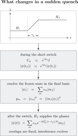
An ideal sudden quench changes $H_i$ to $H_f$ over a time $\tau_q$ too short for appreciable state evolution. The unchanged state is then resolved into final eigenstates, and each component acquires its own phase under the later evolution generated by $H_f$.

Evolution after the Quench

Write the initial vector in the final basis:

$$\lvert\psi_i\rangle = \sum_m c_m\lvert m_f\rangle, \qquad c_m = \langle m_f\vert\psi_i\rangle.$$

For $t\gt0$ and time-independent $H_f$,

$$\lvert\psi(t)\rangle = \sum_m c_m e^{-iE_m^ft/\hbar} \lvert m_f\rangle.$$

The final energy probabilities $\lvert c_m\rvert^2$ are constant, but relative phases evolve. An observable $A$ therefore has expectation value

$$\begin{aligned} \langle A(t)\rangle &= \sum_{m,\ell} c_m^*c_\ell e^{i(E_m^f-E_\ell^f)t/\hbar} \\ &\qquad\times \langle m_f\rvert A\lvert\ell_f\rangle. \end{aligned}$$

Post-quench oscillations are not evidence that the sudden approximation failed. They are the exact evolution of the coherent superposition created by expressing the frozen state in the new basis.

Energy Injected by the Change

For an ideal quench, the mean energy changes because the observable called the Hamiltonian changes:

$$\Delta\overline E = \operatorname{Tr} \left[ \rho_i(H_f-H_i) \right].$$

For an initial eigenstate,

$$\Delta\overline E_n = \langle n_i\rvert H_f\lvert n_i\rangle - E_n^i.$$

The final energy variance is

$$\big(\Delta E_f\big)^2 = \langle H_f^2\rangle_i - \langle H_f\rangle_i^2.$$

The mean change need not be positive for an arbitrary prepared state and protocol. Calling it mean work also requires a stated work convention. For an initial state diagonal in $H_i$, the two-point measurement mean agrees with this energy change, while the full distribution contains the probabilities for individual energy differences. That measurement framework belongs in Work Distributions.

Warm-Up: A Sudden Rotation of a Two-Level Hamiltonian

Consider

$$H_i = -\frac{\Delta}{2}\sigma_z$$

and

$$\begin{aligned} H_f &= -\frac{\Delta}{2} \cos\theta\,\sigma_z \\ &\quad- \frac{\Delta}{2} \sin\theta\,\sigma_x , \\ \Delta &\gt 0. \end{aligned}$$

Prepare the ground state $\lvert g_i\rangle$ of $H_i$. The final ground-state Bloch direction is rotated by angle $\theta$, so

$$\left\lvert \langle g_f\vert g_i\rangle \right\rvert^2 = \cos^2\frac{\theta}{2},$$

and

$$\left\lvert \langle e_f\vert g_i\rangle \right\rvert^2 = \sin^2\frac{\theta}{2}.$$

The mean injected energy is

$$\Delta\overline E = \Delta \sin^2\frac{\theta}{2}.$$

For $\theta=\pi$, the old ground state is the new excited state. For $\theta=0$, the Hamiltonian basis is unchanged and the quench creates no excitation even if a common energy offset changes.

Example: Sudden Expansion of an Infinite Well

Take an initial infinite well on

$$0\lt x\lt L_i$$

and suddenly move the right wall to

$$L_f = \alpha L_i, \qquad \alpha\gt1.$$

The initial eigenfunction is

$$\phi_n^i(x) = \sqrt{\frac{2}{L_i}} \sin\left( \frac{n\pi x}{L_i} \right)$$

for $0\lt x\lt L_i$. Immediately after the expansion, the wavefunction has the same values on the old interval and is zero on the newly opened region:

$$\psi(x,0^+) = \begin{cases} \phi_n^i(x), & 0\lt x\lt L_i,\\ 0, & L_i\lt x\lt L_f. \end{cases}$$

The final eigenfunctions are

$$\phi_m^f(x) = \sqrt{\frac{2}{L_f}} \sin\left( \frac{m\pi x}{L_f} \right).$$

Their overlap amplitudes are

$$\begin{aligned} c_m &= \langle m_f\vert n_i\rangle \\ &= \frac{2}{\sqrt{\alpha}} \int_0^1dy\, \\ &\quad\times \sin\left( \frac{m\pi y}{\alpha} \right) \sin(n\pi y) \\ &= \frac{1}{\sqrt{\alpha}} \frac{ \sin\!\left[\pi(m/\alpha-n)\right] }{ \pi(m/\alpha-n) } \\ &\quad- \frac{1}{\sqrt{\alpha}} \frac{ \sin\!\left[\pi(m/\alpha+n)\right] }{ \pi(m/\alpha+n) } . \end{aligned}$$

At a removable point $m=\alpha n$, the limiting value is

$$c_m = \frac{1}{\sqrt{\alpha}}.$$

The final probabilities are

$$P_m = \lvert c_m\rvert^2, \qquad \sum_{m=1}^{\infty}P_m=1.$$

For a doubling of the well, $\alpha=2$, from the initial ground state $n=1$,

$$\begin{aligned} P_1 &= \frac{32}{9\pi^2} \simeq 0.360, \\ P_2 &= \frac12, \\ P_3 &= \frac{32}{25\pi^2} \simeq 0.130. \end{aligned}$$

All other even-$m$ amplitudes vanish, while higher odd levels carry the remaining probability. The final energies are

$$E_m^f = \frac{\pi^2\hbar^2m^2}{ 2M\alpha^2L_i^2 }.$$

For this ideal expansion, the quadratic-form expectation of the kinetic energy is unchanged at the instant of the quench:

$$\sum_mP_mE_m^f = E_n^i.$$

The energy distribution broadens even though its mean is unchanged. Subsequent interference among the final eigenstates drives nonstationary motion inside the larger well. The stationary spectrum and eigenfunctions themselves belong in Infinite Square Well.

Example: Sudden Change of Oscillator Frequency

Let

$$H(\omega) = \frac{p^2}{2M} + \frac12M\omega^2x^2,$$

and quench

$$\omega_i \longrightarrow \omega_f.$$

Prepare the initial ground state $\lvert0_i\rangle$. It remains the same Gaussian immediately after the switch, but its width does not generally match the final ground-state width. Define

$$r \equiv \frac12 \ln\left( \frac{\omega_f}{\omega_i} \right).$$

In the final oscillator basis, the initial ground state is a squeezed vacuum up to the sign convention used for the squeeze operator. Only even final number states occur:

$$P_{2k+1}=0,$$

and

$$P_{2k} = \frac{(2k)!}{ 2^{2k}(k!)^2 } \frac{\tanh^{2k}r}{\cosh r}.$$

The final ground-state survival probability is

$$\begin{aligned} P_0 &= \frac{1}{\cosh r} \\ &= \frac{ 2\sqrt{\omega_i\omega_f} }{ \omega_i+\omega_f }. \end{aligned}$$

The mean final occupation is

$$\langle N_f\rangle = \sinh^2r = \frac14 \left( \frac{\omega_f}{\omega_i} + \frac{\omega_i}{\omega_f} - 2 \right).$$

Consequently,

$$\begin{aligned} \langle H_f\rangle &= \hbar\omega_f \left( \sinh^2r+\frac12 \right) \\ &= \frac{\hbar}{4} \left( \omega_i + \frac{\omega_f^2}{\omega_i} \right). \end{aligned}$$

Parity, not energy level number, is preserved by the basis overlap because both oscillator Hamiltonians are even under $x\mapsto-x$. The general geometry and number-state expansion of squeezed states belong in Squeezed States: First Encounter.

Finite-Duration Corrections

For a short but nonzero quench, remove the scalar phase and expand the residual evolution:

$$\begin{aligned} e^{i\Phi_q}U_q &= I - \frac{i}{\hbar} \int_{t_i}^{t_f}K(t)\,dt \\ &\quad+ O\!\left( \mathcal A_q^2 \right). \end{aligned}$$

For an initial eigenstate $\lvert n_i\rangle$, the final-basis amplitude is therefore

$$\begin{aligned} e^{i\Phi_q}c_m(\tau_q) &= \langle m_f\vert n_i\rangle \\ &\quad- \frac{i}{\hbar} \int_{t_i}^{t_f} \langle m_f\rvert K(t) \lvert n_i\rangle\,dt \\ &\quad+ O\!\left( \mathcal A_q^2 \right). \end{aligned}$$

The first term is the ideal sudden overlap. The second is actual evolution during the ramp. These amplitudes interfere; one should not add the corresponding probabilities as if they described mutually exclusive processes.

If the first correction is too large, solve the short protocol with the exact time-evolution operator, a Magnus expansion, or direct numerical propagation. The Dyson Expansion for Transition Amplitudes gives the systematic ordered expansion.

A Short Pulse Is Not Always a Frozen Quench

Suppose the Hamiltonian contains a singular pulse,

$$H(t) = H_{\mathrm{reg}}(t) + G\,\delta(t-t_0),$$

with self-adjoint impulse operator $G$. Even though the pulse duration is idealized as zero, its integrated action is finite:

$$\int dt\, G\,\delta(t-t_0) = G.$$

The state changes discontinuously according to

$$\lvert\psi(t_0^+)\rangle = e^{-iG/\hbar} \lvert\psi(t_0^-)\rangle.$$

This is an impulsive unitary kick, not the frozen-state sudden approximation. The relevant small parameter is pulse area divided by $\hbar$, not duration alone. A family of ever shorter pulses whose amplitude grows as $1/\tau_q$ can retain a nontrivial unitary limit.

Sudden and Adiabatic Limits

The sudden and adiabatic approximations answer opposite limiting questions.

Feature	Sudden limit	Adiabatic limit
Protocol scale	short compared with relevant dynamical times	long compared with inverse-gap transition scales
What approximately follows	the fixed state vector	the corresponding instantaneous eigenspace
Final probabilities	overlaps with the final spectral projectors	population remains in the followed eigenspace, up to error
Phase during protocol	usually negligible except for a common phase	dynamical and geometric phases matter
Main danger	finite integrated action or unresolved high-energy modes	small gaps, crossings, and accumulated nonadiabatic coupling

For a large rotation of an eigenbasis, the two limits make sharply different predictions. In the sudden limit the old eigenvector is projected onto many final eigenvectors. In the adiabatic limit an initially isolated eigenstate follows its corresponding instantaneous eigenspace. Runtime diagnostics and leakage estimates are developed in Adiabatic Approximation as a Method, while the theorem-level statement is summarized in the Adiabatic Theorem.

Intermediate protocols are not generally described by interpolating probabilities between the two limits. They require solving the actual dynamics. Landau–Zener Transition is the canonical two-level example.

Degeneracies, Continua, and Large Systems

Degenerate final energies

If $E_a^f$ is degenerate, only

$$p_a^f = \operatorname{Tr} \left( P_a^f\rho_i \right)$$

is basis independent. Probabilities assigned to arbitrary basis vectors inside the eigenspace are meaningful only when an additional commuting observable or later measurement resolves them.

Continuum final spectrum

For generalized final eigenstates $\lvert E,\alpha\rangle$,

$$p_\alpha(E) = \left\lvert \langle E,\alpha\vert\psi_i\rangle \right\rvert^2$$

is a density with respect to the completeness measure. Its dimensions depend on whether the states are normalized in energy, momentum, or a finite box. The normalization dictionary in Density of States in Transition Rates applies here as well, although a sudden projection is not itself a golden-rule rate.

Many-body systems

For an extensive Hamiltonian, a full-system operator norm and global fidelity can scale poorly with volume. A protocol may fail to be globally sudden even when local observables barely change during the switch. High-energy sectors, ultraviolet regularization, locality, and the order of thermodynamic and zero-duration limits can matter. The elementary sudden approximation should not be promoted to a uniform many-body theorem without specifying those controls.

A Reliable Workflow

1. Specify the protocol. State $H_i$, $H_f$, the switching function, and the duration $\tau_q$.
2. Identify the relevant state space. Name the prepared state, occupied energy window, or controlled subspace.
3. Estimate integrated action. Remove scalar phases and test $\mathcal A_q$, a state-specific energy spread, or model-specific transition amplitudes.
4. Check for an impulse. A finite pulse area can produce a nontrivial unitary even as the duration vanishes.
5. Match the Hilbert spaces. If boundaries or domains change, state the embedding of the pre-quench wavefunction into the post-quench problem.
6. Project with spectral projectors. Use $p_a=\operatorname{Tr}(P_a^f\rho_i)$, especially in degenerate sectors.
7. Separate the switch from later evolution. The overlap distribution is set at the quench; later phases generate observable dynamics.
8. Check normalization and energy moments. Verify $\sum_ap_a=1$ or the corresponding continuum integral.
9. Estimate corrections. Compare the finite-ramp amplitude with the ideal overlap before trusting the sudden result quantitatively.

Common Mistakes

• Saying only that the change is “fast.” Fast must be compared with matrix elements, gaps, and the integrated nontrivial action.
• Assuming a large Hamiltonian change invalidates suddenness. A large endpoint difference can still be sudden if the switching interval is sufficiently short on the relevant subspace.
• Assuming every zero-duration protocol leaves the state fixed. A delta-like impulse with finite area applies a unitary kick.
• Projecting before matching Hilbert spaces. Boundary quenches require a clear embedding of the initial state into the final domain.
• Using basis-vector probabilities in a degenerate eigenspace. The invariant object is the probability of the whole spectral projector.
• Calling post-quench oscillations transitions during the quench. They come from phase evolution under $H_f$ after the overlap distribution has been created.
• Confusing overlap probability with a golden-rule rate. A sudden quench can be large and nonperturbative; no long-time continuum limit is involved.
• Ignoring normalization conventions in a continuum. Probability densities change when the generalized eigenstate normalization changes.
• Treating an unbounded-spectrum time-scale slogan as a proof. State domains and high-energy tails require model-specific control.
• Assuming sudden and adiabatic probabilities interpolate linearly. Intermediate dynamics retains phases and interference.

Exercises

Two-level basis rotation

A two-level Hamiltonian is suddenly rotated through an angle $\theta$ as in the warm-up example. The system starts in the initial ground state. Find the final energy probabilities and the final energy variance.

Solution

The probabilities are

$$p_g = \cos^2\frac{\theta}{2}, \qquad p_e = \sin^2\frac{\theta}{2}.$$

The final energies are $-\Delta/2$ and $+\Delta/2$. Hence

$$\langle H_f\rangle = -\frac{\Delta}{2}\cos\theta.$$

Since $H_f^2=(\Delta^2/4)I$,

$$\begin{aligned} \big(\Delta E_f\big)^2 &= \frac{\Delta^2}{4} - \frac{\Delta^2}{4}\cos^2\theta \\ &= \frac{\Delta^2}{4} \sin^2\theta. \end{aligned}$$

The variance vanishes for $\theta=0$ and $\theta=\pi$ because the old ground state is then a definite final energy state.

Doubling an infinite well

For a sudden expansion from $L_i=L$ to $L_f=2L$, starting from $n=1$, calculate $P_1$, $P_2$, and $P_3$. Why is $P_2$ obtained from a limit?

Solution

Substituting $\alpha=2$ and $n=1$ into the overlap formula gives

$$c_1 = \frac{8}{3\pi\sqrt2}, \qquad c_3 = \frac{8}{5\pi\sqrt2}.$$

Therefore

$$P_1 = \frac{32}{9\pi^2}, \qquad P_3 = \frac{32}{25\pi^2}.$$

For $m=2$, the closed form contains a removable $0/0$ term because $m/\alpha=n$. Returning to the integral gives

$$c_2 = \frac{2}{\sqrt2} \int_0^1\sin^2(\pi y)\,dy = \frac{1}{\sqrt2},$$

so

$$P_2=\frac12.$$

The three probabilities sum to approximately $0.990$; higher odd final levels contain the remainder.

Oscillator ground-state survival

An oscillator frequency is suddenly changed from $\omega_i$ to $4\omega_i$. Find the final ground-state probability and the mean final excitation number.

Solution

Here

$$r = \frac12\ln4 = \ln2.$$

The ground-state probability is

$$\begin{aligned} P_0 &= \frac{ 2\sqrt{\omega_i(4\omega_i)} }{ \omega_i+4\omega_i } \\ &= \frac45. \end{aligned}$$

The mean occupation is

$$\begin{aligned} \langle N_f\rangle &= \frac14 \left( 4+\frac14-2 \right) \\ &= \frac{9}{16}. \end{aligned}$$

Although the final ground-state probability is large, the remaining probability occupies an infinite set of even levels and gives a nonzero mean excitation.

Bound a short protocol

On a controlled two-level subspace, suppose

$$\lVert K(t)\rVert \le \frac{\hbar\Omega}{2}$$

throughout a quench of duration $\tau_q$. Give a sufficient suddenness condition and bound the deviation from identity up to a scalar phase.

Solution

The integrated action obeys

$$\begin{aligned} \mathcal A_q &= \frac{1}{\hbar} \int_{t_i}^{t_f} \lVert K(t)\rVert\,dt \\ &\le \frac{\Omega\tau_q}{2}. \end{aligned}$$

Therefore

$$\left\lVert U_q-e^{-i\Phi_q}I \right\rVert \le \frac{\Omega\tau_q}{2}.$$

A sufficient suddenness condition is

$$\Omega\tau_q\ll1.$$

This bound is conservative; a particular state can experience smaller corrections because of symmetry or cancellations.

Distinguish a quench from a kick

Let

$$H_\tau(t) = \frac{1}{\tau} g(t/\tau)G,$$

where $g(s)$ has support on $0\le s\le1$ and

$$\int_0^1g(s)\,ds=1.$$

Find the $\tau\to0$ evolution across the pulse when $G$ is time independent.

Solution

The integrated Hamiltonian is independent of $\tau$:

$$\begin{aligned} \int_0^\tau H_\tau(t)\,dt &= \int_0^\tau \frac{1}{\tau} g(t/\tau)G\,dt \\ &= G. \end{aligned}$$

All pulse Hamiltonians commute because they are proportional to the same $G$, so

$$U_\tau = e^{-iG/\hbar}.$$

The limit is nontrivial rather than the identity. Shrinking duration does not imply a frozen state when the amplitude grows so that the pulse area remains finite.

Degenerate final eigenspace

The final Hamiltonian has a two-dimensional eigenspace with orthonormal basis $\lvert a\rangle,\lvert b\rangle$. Explain which sudden-quench probability is basis independent.

Solution

The spectral projector is

$$P = \lvert a\rangle\langle a\rvert + \lvert b\rangle\langle b\rvert.$$

For an initial density operator $\rho_i$, the probability of the degenerate energy is

$$p = \operatorname{Tr}(P\rho_i).$$

Rotating $\lvert a\rangle,\lvert b\rangle$ within the eigenspace changes the two individual basis probabilities but leaves their sum $p$ invariant. Individual outcomes require an additional observable that resolves a preferred basis inside the degenerate space.

Cross-Links

• Time-Dependent Perturbation Theory and Transitions
• Choosing an Approximation Method
• Time-Dependent Hamiltonians
• Time-Evolution Operator
• Change of Basis
• Probability in Different Bases
• Dyson Expansion for Transition Amplitudes
• Adiabatic Theorem
• Adiabatic Approximation as a Method
• Landau–Zener Transition
• Infinite Square Well
• Squeezed States: First Encounter
• Work Distributions
• Density of States in Transition Rates

References

• L. D. Landau and E. M. Lifshitz, Quantum Mechanics: Non-Relativistic Theory, 3rd ed., Pergamon Press, 1977.
• A. Messiah, Quantum Mechanics, Vol. II, North-Holland, 1962.
• C. Cohen-Tannoudji, B. Diu, and F. Laloë, Quantum Mechanics, Wiley, 1977.
• J. J. Sakurai and J. Napolitano, Modern Quantum Mechanics, 3rd ed., Cambridge University Press, 2020.
• D. J. Griffiths and D. F. Schroeter, Introduction to Quantum Mechanics, 3rd ed., Cambridge University Press, 2018.
• A. Polkovnikov, K. Sengupta, A. Silva, and M. Vengalattore, “Colloquium: Nonequilibrium dynamics of closed interacting quantum systems,” Reviews of Modern Physics 83, 863–883 (2011).