Infinite Square Well

The infinite square well is the canonical model of boundary quantization. A particle of mass $m$ is confined to the interval $0\lt x\lt L$ by impenetrable walls. Inside the well the particle is free; the quantization of energy comes entirely from the boundary conditions.

The potential is

$$V(x)= \begin{cases} 0, & 0\lt x\lt L,\\ \infty, & x\le 0 \text{ or } x\ge L. \end{cases}$$

The wavefunction vanishes outside the well and satisfies

$$\psi(0)=0, \qquad \psi(L)=0.$$

The symbol $\infty$ is shorthand for an ideal constraint, not an ordinary real-valued potential to substitute into algebra. The clean mathematical model is the kinetic-energy operator on the interval with Dirichlet endpoint conditions. A very deep finite well approaches this model for low-lying states, but its wavefunctions retain evanescent tails and its spectrum is never literally identical at finite depth.

Hamiltonian And Hilbert Space

The Hilbert space is $L^2([0,L])$ with inner product

$$\langle \phi|\psi\rangle =\int_0^L \phi^*(x)\psi(x)\,dx.$$

Inside the well, the Hamiltonian is the kinetic-energy operator

$$\hat H =-\frac{\hbar^2}{2m}\frac{d^2}{dx^2},$$

with the hard-wall boundary conditions above. The boundary conditions are not optional; they define the domain of the Hamiltonian for this problem.

For the standard self-adjoint realization, the domain consists of sufficiently regular functions whose endpoint values vanish. In Sobolev notation,

$$\mathcal D(\hat H) =H^2(0,L)\cap H_0^1(0,L).$$

Integration by parts then gives

$$\langle\psi|\hat H|\psi\rangle =\frac{\hbar^2}{2m} \int_0^L\lvert\psi'(x)\rvert^2\,dx \ge0.$$

The Hamiltonian is therefore nonnegative. It also has a compact resolvent on this finite interval, so its spectrum consists of discrete eigenvalues tending to infinity.

Stationary Equation

The time-independent Schrödinger equation inside the well is

$$-\frac{\hbar^2}{2m}\frac{d^2\psi}{dx^2} =E\psi.$$

For positive energy, write

$$k=\frac{\sqrt{2mE}}{\hbar}.$$

The general solution inside the well is

$$\psi(x)=A\sin(kx)+B\cos(kx).$$

The boundary condition at $x=0$ gives $B=0$. The boundary condition at $x=L$ gives

$$A\sin(kL)=0.$$

For a nonzero wavefunction,

$$kL=n\pi, \qquad n=1,2,3,\ldots$$

The allowed energies are therefore

$$E_n =\frac{\hbar^2k_n^2}{2m} =\frac{n^2\pi^2\hbar^2}{2mL^2}.$$

The cases $E\le0$ produce no additional states. At $E=0$, the solution $A+Bx$ cannot vanish at both endpoints unless it is zero. At $E\lt0$, a hyperbolic-sine solution satisfying the left wall cannot also vanish at the right wall. Positivity of $\hat H$ gives the same conclusion immediately.

It is useful to define the natural box scales

$$k_1=\frac{\pi}{L}, \qquad p_1=\frac{\pi\hbar}{L}, \qquad E_1=\frac{\pi^2\hbar^2}{2mL^2}.$$

Then $k_n=nk_1$, $p_n=np_1$ as a kinetic-energy scale, and $E_n=n^2E_1$.

Normalized Eigenfunctions

The normalized eigenfunctions are

$$\psi_n(x) =\sqrt{\frac{2}{L}}\sin\frac{n\pi x}{L}, \qquad n=1,2,3,\ldots$$

They satisfy

$$\int_0^L \psi_m^*(x)\psi_n(x)\,dx =\delta_{mn}.$$

For $m=n$, normalization follows from

$$\int_0^L\sin^2\frac{n\pi x}{L}\,dx =\frac{L}{2}.$$

For $m\ne n$, orthogonality can be checked with trigonometric identities. More generally, self-adjointness gives

$$(E_n-E_m) \langle\psi_m|\psi_n\rangle=0,$$

so distinct-energy eigenfunctions are orthogonal. Each eigenvalue is nondegenerate: once $\psi(0)=0$ fixes the cosine coefficient, $\psi(L)=0$ leaves only one sine solution up to normalization and phase.

Orthogonality and Completeness

The eigenfunctions form a complete basis for $L^2([0,L])$. Boundary values distinguish the Hamiltonian domain from the full Hilbert space; an arbitrary square-integrable state need not possess pointwise endpoint values. Every initial state in the Hilbert space nevertheless has the norm-convergent expansion

$$\psi(x,0)=\sum_{n=1}^{\infty}c_n\psi_n(x), \qquad c_n=\int_0^L \psi_n^*(x)\psi(x,0)\,dx.$$

Completeness can be expressed distributionally as

$$\sum_{n=1}^{\infty} \psi_n(x)\psi_n^*(x') =\delta(x-x'), \qquad 0\lt x,x'\lt L.$$

For a normalized initial state, Parseval’s identity gives

$$\sum_{n=1}^{\infty}\lvert c_n\rvert^2=1.$$

Time evolution is then

$$\psi(x,t) =\sum_{n=1}^{\infty} c_n\psi_n(x)e^{-iE_nt/\hbar}.$$

The expansion converges in Hilbert-space norm for every square-integrable initial state. Pointwise convergence at a cusp or discontinuity is a separate Fourier-analysis question, and applying $\hat H$ term by term requires stronger regularity than merely having finite norm.

Physical Lessons

The infinite square well teaches several durable lessons.

Energy is quantized by boundary conditions. The particle is free inside the box, but only wavelengths fitting the interval are allowed:

$$\lambda_n=\frac{2L}{n}.$$

The ground-state energy is not zero:

$$E_1=\frac{\pi^2\hbar^2}{2mL^2}.$$

Confinement costs kinetic energy. Making $L$ smaller raises all energies as $1/L^2$.

The $n$th eigenfunction has $n-1$ interior nodes. Higher energy corresponds to shorter wavelength and more oscillation.

The nodes occur at

$$x_j=\frac{jL}{n}, \qquad j=1,2,\ldots,n-1.$$

This realizes the one-dimensional nodal theorem: ordering the nondegenerate bound states by increasing energy, the $n$th state has exactly $n-1$ interior zeros. The adjacent level spacing is

$$E_{n+1}-E_n =(2n+1)E_1,$$

so the spectrum becomes more widely spaced in energy as $n$ increases. It is not an equally spaced ladder.

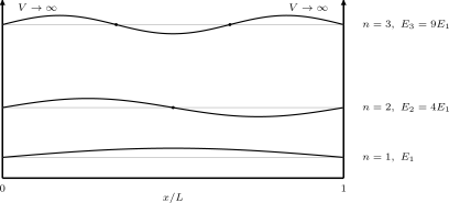
The first three eigenfunctions, offset by their energies. The levels scale as $E_n=n^2E_1$, and the marked interior zeros show the $n-1$ node rule. Wavefunction amplitudes are schematic and are not plotted on the energy scale.

Expectation Values

For every stationary eigenstate,

$$\langle x\rangle_n=\frac{L}{2}.$$

The second moment and variance are

$$\begin{aligned} \langle x^2\rangle_n &=L^2 \left( \frac{1}{3} -\frac{1}{2n^2\pi^2} \right),\\ (\Delta x)^2_n &=L^2 \left( \frac{1}{12} -\frac{1}{2n^2\pi^2} \right). \end{aligned}$$

Formally applying $-i\hbar,d/dx$ gives

$$\langle p\rangle_n=0,$$

because the real eigenfunction vanishes at both endpoints. The robust kinetic-energy statement is

$$\langle p^2\rangle_n =2mE_n =\frac{n^2\pi^2\hbar^2}{L^2}.$$

Thus

$$\Delta p_n=\frac{n\pi\hbar}{L}.$$

Consequently,

$$(\Delta x)_n(\Delta p)_n =\frac{\hbar}{2} \sqrt{\frac{n^2\pi^2}{3}-2} \ge\frac{\hbar}{2}.$$

Because $\psi_n$ is an energy eigenstate,

$$\langle H\rangle_n=E_n, \qquad \Delta H_n=0.$$

There is an operator-domain subtlety behind the momentum notation. The derivative operator $-i\hbar,d/dx$ with Dirichlet conditions at both ends is symmetric but not self-adjoint; its self-adjoint interval realizations instead relate endpoint values by a phase. The box Hamiltonian and $p^2=2mH$ are well-defined, but an intrinsic sharp momentum observable for the hard-wall interval requires more care than the formal expectation above suggests.

Likewise, writing a sine as two complex exponentials does not mean a release-and-measure experiment yields only the two momenta $\pm n\pi\hbar/L$. Once regarded as a compactly supported full-line wavefunction after the walls are removed, its Fourier transform is a continuous distribution broadened by the finite spatial support. This distinction is developed alongside Hermitian vs Self-Adjoint Operators.

The elementary lesson remains valid: a vanishing first momentum moment does not imply vanishing kinetic energy.

Centered-Well Parity Form

For a well of the same width centered at the origin, $-L/2\lt x\lt L/2$, the potential is symmetric. Up to an irrelevant sign for individual states, the normalized eigenfunctions can be written

$$\psi_n^{(c)}(x) =\sqrt{\frac{2}{L}} \begin{cases} \cos(n\pi x/L), & n\text{ odd},\\ \sin(n\pi x/L), & n\text{ even}. \end{cases}$$

States with odd $n$ are parity even, and states with even $n$ are parity odd. The energies remain $E_n=n^2E_1$. The centered form is often better for discussing parity and selection rules, while the interval $0\lt x\lt L$ form is convenient for direct boundary-condition calculations. They describe equivalent physics after the shift $x\mapsto x+L/2$ and harmless state-dependent phase choices.

Superpositions Are Not Stationary

Each energy eigenstate has a time-independent probability density. A superposition generally does not. For example,

$$\psi(x,t) =c_1\psi_1(x)e^{-iE_1t/\hbar} +c_2\psi_2(x)e^{-iE_2t/\hbar}$$

has interference terms oscillating at angular frequency

$$\omega_{21}=\frac{E_2-E_1}{\hbar} =\frac{3\pi^2\hbar}{2mL^2}.$$

The probability density can slosh back and forth even though the Hamiltonian is time independent.

For the equal superposition $c_1=c_2=1/\sqrt2$, the real spatial eigenfunctions give

$$\lvert\psi(x,t)\rvert^2 =\frac{1}{2}\left(\psi_1^2+\psi_2^2\right) +\psi_1\psi_2\cos(\omega_{21}t).$$

The interference term changes sign over a cycle. Since

$$\langle1|x|2\rangle =-\frac{16L}{9\pi^2},$$

the packet center oscillates as

$$\langle x\rangle_t =\frac{L}{2} -\frac{16L}{9\pi^2} \cos(\omega_{21}t).$$

Its energy distribution is time independent:

$$\langle H\rangle =\frac{E_1+E_2}{2} =\frac{5}{2}E_1, \qquad \Delta H =\frac{E_2-E_1}{2} =\frac{3}{2}E_1.$$

The density oscillation period is

$$T_{12} =\frac{2\pi}{\omega_{21}} =\frac{4mL^2}{3\pi\hbar}.$$

Exact Revivals

Because every energy is an integer square times $E_1$, an arbitrary state revives exactly after

$$T_{\mathrm{rev}} =\frac{2\pi\hbar}{E_1} =\frac{4mL^2}{\pi\hbar}.$$

Indeed,

$$e^{-iE_nT_{\mathrm{rev}}/\hbar} =e^{-i2\pi n^2} =1$$

for every $n$. At half this time, the phase is $(-1)^n$ and the initial wavefunction is reconstructed as its mirror image about $L/2$, up to a global phase. Fractional revival structures can occur at rational fractions of $T_{\mathrm{rev}}$.

For a packet concentrated around a large quantum number $n_0$, the associated classical round-trip period is approximately

$$T_{\mathrm{cl}} =\frac{2L}{p_{n_0}/m} =\frac{2mL^2}{n_0\pi\hbar},$$

and $T_{\mathrm{rev}}/T_{\mathrm{cl}}=2n_0$. The separation of these scales explains why a localized packet can undergo many approximately classical bounces before its fully quantum revival.

Worked Example: A Triangular Initial State

Consider the continuous, symmetric initial wavefunction

$$\psi_{\triangle}(x,0) =A \begin{cases} x, & 0\le x\le L/2,\\ L-x, & L/2\le x\le L. \end{cases}$$

Normalization gives

$$1 =2\lvert A\rvert^2 \int_0^{L/2}x^2\,dx =\frac{\lvert A\rvert^2L^3}{12},$$

so a convenient phase choice is

$$A=\frac{2\sqrt3}{L^{3/2}}.$$

The expansion coefficients are

$$\begin{aligned} c_n &=\int_0^L\psi_n(x)\psi_{\triangle}(x,0)\,dx\\ &=\frac{4\sqrt6}{\pi^2n^2} \sin\frac{n\pi}{2}. \end{aligned}$$

Even $n$ vanish because the triangle is even about the center whereas the even-$n$ eigenfunctions are parity odd in centered coordinates. The alternating sign of the odd-$n$ coefficients reconstructs the cusp at $x=L/2$. Normalization is checked by

$$\sum_{n=1}^{\infty}\lvert c_n\rvert^2 =\frac{96}{\pi^4} \sum_{\substack{n=1\\n\text{ odd}}}^{\infty} \frac{1}{n^4} =1.$$

Its exact evolution is

$$\psi_{\triangle}(x,t) =\sum_{n=1}^{\infty} c_n\psi_n(x) e^{-in^2E_1t/\hbar}.$$

The coefficient decay also diagnoses regularity. Since $c_n\sim n^{-2}$,

$$\langle H\rangle =\sum_n\lvert c_n\rvert^2E_n =\frac{12}{\pi^2}E_1 =\frac{6\hbar^2}{mL^2}$$

is finite, but $\langle H^2\rangle$ diverges. The state lies in the energy quadratic-form domain but not in the operator domain of $H$: its first derivative has a jump at the apex, so its second derivative contains a delta distribution. Unitary evolution is still well-defined because the initial wavefunction is an element of the Hilbert space.

Classical Comparison

Classically, a particle in a box moves at constant speed and bounces off the walls. Quantum mechanically, energy eigenstates are standing waves with no definite direction of motion. A localized wave packet can approximate a bouncing classical particle for suitable states and times, but exact energy eigenstates do not trace classical trajectories. The large-$n$ and coarse-graining aspects are discussed in Correspondence Principle.

For one energy eigenstate,

$$\lvert\psi_n(x)\rvert^2 =\frac{1}{L} \left[ 1-\cos\left(\frac{2n\pi x}{L}\right) \right].$$

The classical time-averaged position density is uniform, $1/L$. The quantum density does not converge pointwise to that value as $n\to\infty$; its oscillations become increasingly rapid. Against a detector response or test function smooth on scales much larger than $L/n$, the cosine term averages away. Classical agreement is therefore weak or coarse-grained, not pointwise.

The relative spacing of neighboring energies behaves as

$$\frac{E_{n+1}-E_n}{E_n} =\frac{2n+1}{n^2} \sim\frac{2}{n}.$$

At large $n$, nearby levels are close on the scale of the energy even though their absolute separation grows. Superpositions spanning many nearby levels can then form localized packets with an approximately classical bounce period. Nodes, interference, collapse, and revival remain quantum features beyond that approximation.

Numerical Benchmark

Place $N$ interior grid points at $x_j=jh$, where $h=L/(N+1)$, and fix the omitted endpoint values to zero. The centered second-difference Hamiltonian is

$$H_h =\frac{\hbar^2}{2mh^2} \begin{pmatrix} 2 & -1 & 0 & \cdots & 0\\ -1 & 2 & -1 & \ddots & \vdots\\ 0 & -1 & 2 & \ddots & 0\\ \vdots & \ddots & \ddots & \ddots & -1\\ 0 & \cdots & 0 & -1 & 2 \end{pmatrix}.$$

This matrix has analytic discrete eigenpairs

$$\begin{aligned} E_n^{(h)} &=\frac{\hbar^2}{mh^2} \left[ 1-\cos\left(\frac{n\pi}{N+1}\right) \right],\\ v_j^{(n)} &=\sqrt{\frac{2}{N+1}} \sin\left(\frac{n\pi j}{N+1}\right), \end{aligned}$$

for $n=1,\ldots,N$. At fixed $n$ and increasing $N$,

$$E_n^{(h)} =E_n \left[ 1-\frac{n^2\pi^2}{12(N+1)^2} +O\left((N+1)^{-4}\right) \right].$$

The second-order stencil therefore approaches the continuum energy from below with an $O(h^2)$ error. The matrix eigenvectors have Euclidean norm one; sampled continuum wavefunctions are recovered through $\psi_n(x_j)\approx v_j^{(n)}/\sqrt h$. A trustworthy implementation should reproduce the $1:4:9$ low-level ratios, node counts, orthogonality, and this convergence law.

Common Mistakes

• Allowing $n=0$ as a physical eigenstate. It gives the zero wavefunction, not a particle state.
• Treating $V=\infty$ as an ordinary number rather than defining the Dirichlet interval problem.
• Forgetting the normalization factor $\sqrt{2/L}$.
• Requiring $\psi'$ to vanish at a hard wall; only the Dirichlet value $\psi$ vanishes.
• Saying the particle has zero kinetic energy because $V=0$ inside the well.
• Treating finite walls as if they imposed $\psi=0$.
• Confusing $\langle p\rangle=0$ with $\langle p^2\rangle=0$.
• Treating $-i\hbar d/dx$ with two Dirichlet endpoints as a self-adjoint momentum operator.
• Assuming the two-exponential identity for a sine gives two delta-function outcomes after a release momentum measurement.
• Calling the $n^2$ spectrum equally spaced.
• Expecting $\lvert\psi_n\rvert^2$ to converge pointwise to the classical uniform density at large $n$.
• Assuming every square-integrable expansion lies in the operator domain or has finite energy variance.
• Thinking an energy eigenstate describes a classical particle bouncing between walls.

Where This Is Used

• Boundary Conditions explains hard-wall conditions.
• Propagators and Boundary Conditions derives the hard-wall spectral and image kernels.
• Time-Independent Schrödinger Equation gives the eigenvalue-problem framework.
• Periodic Functions and Fourier Series compares periodic modes with the sine modes used by hard-wall boxes.
• Sturm–Liouville Theory explains why these eigenfunctions are orthogonal and complete.
• Matrix Diagonalization uses the well as a benchmark for numerical spectra.
• Normalization Conventions relates grid-vector and continuum normalizations.
• Finite Square Well relaxes the infinite-wall idealization.
• Sudden Approximation uses a rapid well expansion to illustrate projection onto a changed boundary-condition basis.

References

• D. J. Griffiths and D. F. Schroeter, Introduction to Quantum Mechanics, 3rd ed., Cambridge University Press, 2018.
• R. Shankar, Principles of Quantum Mechanics, 2nd ed., Springer, 1994.
• C. Cohen-Tannoudji, B. Diu, and F. Laloë, Quantum Mechanics, Wiley, 1977.
• E. Merzbacher, Quantum Mechanics, 3rd ed., Wiley, 1998.
• R. W. Robinett, “Quantum wave packet revivals,” Physics Reports 392, 1–119 (2004), doi:10.1016/j.physrep.2003.11.002.

Exercises

1. Normalize $\psi_n(x)=A\sin(n\pi x/L)$ on $0\lt x\lt L$.

Solution

Use

$$\int_0^L \sin^2\frac{n\pi x}{L}\,dx=\frac{L}{2}.$$

Then

$$1=|A|^2\frac{L}{2},$$

so $A=\sqrt{2/L}$ up to an overall phase.

2. Compute the formal differential-operator expectation $\langle\psi_n|-i\hbar d/dx|\psi_n\rangle$. Why does this calculation alone not establish a self-adjoint momentum observable for the hard-wall box?

Solution

Use $\hat p=-i\hbar d/dx$:

$$\langle p\rangle_n =-i\hbar\int_0^L\psi_n(x)\frac{d\psi_n}{dx}\,dx.$$

Since $\psi_n d\psi_n/dx=(1/2)d(\psi_n^2)/dx$,

$$\langle p\rangle_n =-\frac{i\hbar}{2}\left[\psi_n^2(x)\right]_0^L=0,$$

because $\psi_n(0)=\psi_n(L)=0$.

This vanishing matrix element is a valid formal calculation, but self-adjointness is a statement about an operator and its full domain, not one expectation value. The first-derivative operator with Dirichlet conditions at both endpoints does not have the same domain as its adjoint. Its self-adjoint interval extensions use phase-related endpoint values, which are incompatible with the two hard-wall conditions except for the zero function.

3. How does the ground-state energy change if the box length is doubled?

Solution

The ground-state energy is

$$E_1=\frac{\pi^2\hbar^2}{2mL^2}.$$

Replacing $L$ by $2L$ gives $E_1/4$. Doubling the box length lowers the ground-state energy by a factor of four.

4. Derive $\langle x^2\rangle_n$ and $(\Delta x)^2_n$ for the standard eigenstate on $[0,L]$.

Solution

Using $\sin^2u=(1-\cos2u)/2$,

$$\begin{aligned} \langle x^2\rangle_n &=\frac{2}{L} \int_0^L x^2 \sin^2\frac{n\pi x}{L}\,dx\\ &=\frac{1}{L} \int_0^L x^2\,dx -\frac{1}{L} \int_0^L x^2 \cos\frac{2n\pi x}{L}\,dx. \end{aligned}$$

The two integrals are

$$\int_0^Lx^2\,dx=\frac{L^3}{3}, \qquad \int_0^Lx^2\cos\frac{2n\pi x}{L}\,dx =\frac{L^3}{2n^2\pi^2}.$$

Therefore

$$\langle x^2\rangle_n =L^2 \left( \frac13-\frac{1}{2n^2\pi^2} \right).$$

Since $\langle x\rangle_n=L/2$,

$$(\Delta x)^2_n =L^2 \left( \frac1{12}-\frac{1}{2n^2\pi^2} \right).$$

5. Derive the expansion coefficients of the normalized triangular state on this page. Use them to calculate its mean energy.

Solution

With $A=2\sqrt3/L^{3/2}$, reflection about $L/2$ makes the two half-interval contributions equal for odd $n$ and opposite for even $n$. Thus even coefficients vanish. For odd $n$,

$$\begin{aligned} c_n &=2A\sqrt{\frac2L} \int_0^{L/2}x \sin\frac{n\pi x}{L}\,dx\\ &=2A\sqrt{\frac2L} \frac{L^2}{n^2\pi^2} \sin\frac{n\pi}{2}\\ &=\frac{4\sqrt6}{n^2\pi^2} \sin\frac{n\pi}{2}. \end{aligned}$$

Since $E_n=n^2E_1$,

$$\begin{aligned} \langle H\rangle &=\frac{96E_1}{\pi^4} \sum_{\substack{n=1\\n\text{ odd}}}^{\infty} \frac{1}{n^2}\\ &=\frac{96E_1}{\pi^4} \frac{\pi^2}{8} =\frac{12E_1}{\pi^2}. \end{aligned}$$

6. Show that at $T_{\mathrm{rev}}/2$ an arbitrary initial state is reconstructed as a mirror image about the center, up to a global phase.

Solution

At half the revival time,

$$e^{-iE_nT_{\mathrm{rev}}/(2\hbar)} =e^{-i\pi n^2} =(-1)^n.$$

The sine eigenfunctions obey

$$\begin{aligned} \psi_n(L-x) &=\sqrt{\frac2L} \sin\left(n\pi-\frac{n\pi x}{L}\right)\\ &=(-1)^{n+1}\psi_n(x). \end{aligned}$$

Hence $(-1)^n\psi_n(x)=-\psi_n(L-x)$ for every $n$. Applying this relation term by term to the spectral expansion gives

$$\psi(x,T_{\mathrm{rev}}/2) =-\psi(L-x,0).$$

The minus sign is a global phase and has no effect on the probability density.