Hermitian vs Self-Adjoint Operators

For a finite matrix, Hermitian and self-adjoint mean the same thing:

$$A^\dagger=A.$$

For an unbounded operator on an infinite-dimensional Hilbert space, the same symbols can hide different domains. A differential expression may be formally Hermitian, an operator built from it may be symmetric on one domain, and only a particular domain choice may make it self-adjoint.

The short rule is:

Symmetric means the inner-product identity holds on the chosen domain. Self-adjoint means the operator and its adjoint have the same action and the same domain.

This page gives the precision needed in Core Formalism, including the detailed interval boundary-condition example. The canonical operator-theoretic treatment of closures, deficiency indices, range tests, and spectral and dynamical consequences is Self-Adjoint Operators. The Mathematical Toolkit pages retain the prerequisite vocabulary for domains and adjoints.

Finite-Dimensional Case

Let $\mathcal H=\mathbb C^d$. Every linear operator is bounded and defined on all of $\mathcal H$:

$$\mathcal D(A)=\mathcal H.$$

Its adjoint is also defined on all of $\mathcal H$. Therefore there is no domain mismatch to track, and the conditions

$$\langle\phi|A\psi\rangle = \langle A\phi|\psi\rangle$$

for all vectors and

$$A^\dagger=A$$

are equivalent.

In an orthonormal basis,

$$[A^\dagger] = \left([A]^*\right)^{\mathsf T},$$

so the familiar matrix condition is

$$A_{mn}=A_{nm}^*.$$

A Hermitian matrix has:

• real eigenvalues;
• orthogonal eigenspaces for distinct eigenvalues;
• an orthonormal eigenbasis;
• a spectral decomposition by orthogonal projectors;
• real expectation values in every state.

Thus “observables are represented by Hermitian matrices” is correct for finite-level systems, spin matrices, and ordinary quantum-information models. See Hermitian Operators for the matrix theory.

Why Infinite Dimension Is Different

An operator is not merely a formula. It includes a domain:

$$A:\mathcal D(A)\subseteq\mathcal H \longrightarrow\mathcal H.$$

For an unbounded operator, $\mathcal D(A)$ is generally a proper dense subspace. Position, momentum, and differential Hamiltonians do not act on every square-integrable function.

For example, the formal expression

$$-i\hbar\frac{d}{dx}$$

does not specify:

• which interval or manifold $x$ belongs to;
• which square-integrable functions possess the required derivative;
• which endpoint or matching conditions hold;
• whether the output remains in the Hilbert space.

Changing any of these choices can change the operator, its adjoint, and its spectrum.

The Adjoint Has Its Own Domain

Let $A$ be densely defined. A vector $|\phi\rangle$ belongs to $\mathcal D(A^\dagger)$ when there is a vector $|\eta\rangle\in\mathcal H$ such that

$$\langle\phi|A\psi\rangle = \langle\eta|\psi\rangle$$

for every $|\psi\rangle\in\mathcal D(A)$. The adjoint is then defined by

$$A^\dagger|\phi\rangle=|\eta\rangle.$$

The representing vector $|\eta\rangle$ is unique because $\mathcal D(A)$ is dense. Equivalently, the map

$$|\psi\rangle \longmapsto \langle\phi|A\psi\rangle$$

must be continuous with respect to the Hilbert-space norm on $\mathcal D(A)$.

The key point is:

$$\mathcal D(A^\dagger) \quad\text{need not equal}\quad \mathcal D(A).$$

The adjoint is therefore another operator with its own domain, not merely a formal conjugate-transpose symbol. See Adjoint Operators for the construction.

Symmetric Operators

A densely defined operator $A$ is symmetric when

$$\langle\phi|A\psi\rangle = \langle A\phi|\psi\rangle$$

for all $|\phi\rangle,|\psi\rangle\in\mathcal D(A)$.

In operator-inclusion notation,

$$A\subseteq A^\dagger.$$

This means

$$\mathcal D(A)\subseteq\mathcal D(A^\dagger)$$

and

$$A^\dagger|\psi\rangle=A|\psi\rangle \qquad \text{for every }|\psi\rangle\in\mathcal D(A).$$

Symmetry implies real expectation values on the domain:

$$\begin{aligned} \langle\psi|A\psi\rangle^* &=\langle A\psi|\psi\rangle\\ &=\langle\psi|A\psi\rangle. \end{aligned}$$

This is necessary for a real-valued observable, but it is not sufficient for the full sharp-observable framework. A symmetric operator can have an adjoint defined on more vectors than the original operator.

Self-Adjoint Operators

An operator is self-adjoint when it equals its adjoint as an operator:

$$A=A^\dagger.$$

This statement contains two conditions:

$$\mathcal D(A)=\mathcal D(A^\dagger)$$

and, on that common domain,

$$A|\psi\rangle=A^\dagger|\psi\rangle.$$

Every self-adjoint operator is symmetric. The converse is false for unbounded operators.

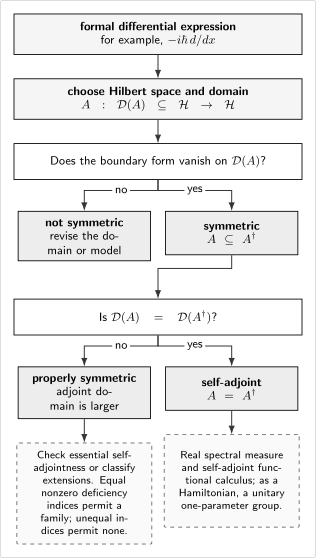
The same local expression can define different operators. Symmetry constrains the boundary form on a chosen domain; self-adjointness additionally requires that no larger adjoint domain remains.

Formal Hermiticity

A formal adjoint is obtained by algebraic conjugation and integration by parts while temporarily suppressing boundary terms. A differential expression is often called formally Hermitian when it equals this formal adjoint.

For example,

$$-i\hbar\frac{d}{dx}$$

has the expected formal adjoint expression. But formal equality says nothing by itself about which boundary terms vanish or which domains agree.

The phrases form a progression of increasingly complete checks:

1. Formally Hermitian: the differential expression matches its formal adjoint.
2. Symmetric: the boundary form vanishes for every pair in the chosen operator domain.
3. Self-adjoint: the symmetric operator has the same domain as its Hilbert- space adjoint.
4. Essentially self-adjoint: a symmetric operator has a unique self-adjoint closure.

Formal Hermiticity by itself is not yet an operator property because no domain has been supplied. Once a domain is chosen, the boundary form determines whether the resulting operator is symmetric; equality with the adjoint domain then determines self-adjointness. Skipping those steps is the common error.

Boundary Forms

Integration by parts exposes the domain dependence. For momentum on $[0,L]$,

$$P=-i\hbar\frac{d}{dx},$$

one finds for sufficiently regular functions

$$\begin{aligned} \langle\phi|P\psi\rangle -\langle P\phi|\psi\rangle &= -i\hbar \left[ \phi^*(x)\psi(x) \right]_0^L\\ &= -i\hbar\phi^*(L)\psi(L)\\ &\quad +i\hbar\phi^*(0)\psi(0). \end{aligned}$$

The right-hand side is the boundary form. A proposed domain makes $P$ symmetric only when this form vanishes for every allowed pair $\phi,\psi$.

For a second-order expression such as

$$H_0 = -\frac{\hbar^2}{2m}\frac{d^2}{dx^2},$$

the corresponding boundary form is

$$\begin{aligned} &\langle\phi|H_0\psi\rangle -\langle H_0\phi|\psi\rangle\\ &\qquad= -\frac{\hbar^2}{2m} \left[ \phi^*\psi' -\phi'^*\psi \right]_0^L. \end{aligned}$$

Dirichlet, Neumann, periodic, and Robin-type conditions can cancel this form in different ways. They need not define the same self-adjoint operator or the same spectrum.

Momentum on an Interval

Let

$$\mathcal H=L^2([0,L])$$

and begin with the momentum expression

$$P=-i\hbar\frac{d}{dx}.$$

Dirichlet domain: symmetric but not self-adjoint

Consider

$$\mathcal D_0(P) = \left\lbrace \begin{gathered} \psi\in H^1([0,L])\\[-2pt] \psi(0)=\psi(L)=0 \end{gathered} \right\rbrace.$$

The boundary form vanishes because both endpoint values vanish. Therefore $P$ is symmetric on $\mathcal D_0(P)$.

However, testing against every Dirichlet $\psi$ imposes no endpoint condition on vectors in the adjoint domain. One obtains a larger adjoint domain, essentially

$$\mathcal D(P^\dagger)=H^1([0,L]).$$

Hence

$$\mathcal D_0(P) \subsetneq \mathcal D(P^\dagger),$$

so this momentum operator is not self-adjoint.

Phase-twisted domains: self-adjoint

For any fixed $\theta\in[0,2\pi)$, define

$$\mathcal D_\theta(P) = \left\lbrace \begin{gathered} \psi\in H^1([0,L])\\[-2pt] \psi(L)=e^{i\theta}\psi(0) \end{gathered} \right\rbrace.$$

If $\phi$ and $\psi$ satisfy the same condition, then

$$\begin{aligned} \phi^*(L)\psi(L) &= e^{-i\theta}\phi^*(0) e^{i\theta}\psi(0)\\ &= \phi^*(0)\psi(0), \end{aligned}$$

so the boundary form vanishes. Moreover, requiring the form to vanish against every $\psi\in\mathcal D_\theta(P)$ forces an adjoint-domain vector $\phi$ to obey the same phase relation. Thus

$$\mathcal D(P^\dagger) = \mathcal D_\theta(P)$$

for this realization, and $P_\theta$ is self-adjoint.

Its normalized eigenfunctions are

$$\psi_n(x) = \frac{1}{\sqrt L} \exp\left(i k_nx\right),$$

where

$$k_n = \frac{2\pi n+\theta}{L}, \qquad p_n = \hbar k_n, \qquad n\in\mathbb Z.$$

Different $\theta$ give different self-adjoint operators and shifted spectra, even though the local expression is unchanged.

Symmetric Does Not Mean “Almost Good Enough”

It is tempting to treat a symmetric operator as a self-adjoint operator with a minor technical defect. That framing is misleading. The missing domain information controls whether:

• the spectrum is the real spectral set of a sharp observable;
• a projection-valued spectral measure exists;
• $f(A)$ is defined by the self-adjoint functional calculus;
• a Hamiltonian generates unitary evolution for all real times;
• boundary probability flux is conserved under the proposed dynamics.

Symmetry supplies real expectation values on a test domain. Self-adjointness supplies the complete operator needed by the spectral and dynamical theory.

Essentially Self-Adjoint Operators

A symmetric operator $A_0$ is essentially self-adjoint when its closure $\overline{A_0}$ is self-adjoint:

$$\overline{A_0} = A_0^\dagger.$$

Equivalently, the starting operator determines a unique self-adjoint extension. This is useful because differential operators are often introduced first on a convenient dense core such as smooth compactly supported functions.

If $A_0$ is essentially self-adjoint, no additional boundary parameter is needed to select the mathematical realization. If it is not, two mathematical possibilities must be distinguished:

• equal nonzero deficiency indices permit a family of self-adjoint extensions;
• unequal deficiency indices permit no self-adjoint extension.

Additional physical structure may select one member of an allowed family. The classification uses deficiency spaces and lies beyond this Core page. The mathematical entry point is Symmetric versus Self-Adjoint Operators.

Self-Adjoint Extensions

A self-adjoint extension $\widetilde A$ of a symmetric $A$ satisfies

$$A\subseteq\widetilde A = \widetilde A^\dagger.$$

The extension retains the original action on $\mathcal D(A)$ while enlarging the domain. For differential operators, extension parameters are often boundary conditions.

The interval momentum example has a one-parameter family $P_\theta$. The Dirichlet-domain momentum operator $P_{\mathrm D}$ is contained in each:

$$P_{\mathrm D} \subset P_\theta.$$

There is no contradiction in having several self-adjoint extensions. The starting symmetric operator did not yet encode a complete physical boundary condition. Choosing an extension completes the model.

Different extensions can have different spectra and dynamics. They are not different gauges or different matrix representations of one already-specified operator.

Why Self-Adjointness Matters for Observables

A standard sharp observable is represented by a self-adjoint operator. The spectral theorem provides a projection-valued measure

$$\Delta \longmapsto P_A(\Delta)$$

on real outcome sets. For a normalized state,

$$\Pr(A\in\Delta) = \langle\psi|P_A(\Delta)|\psi\rangle.$$

This framework handles discrete, continuous, and mixed spectra. A merely symmetric operator does not automatically carry the required self-adjoint spectral measure.

Real expectation values are therefore not the whole observable criterion. They are a local quadratic-form property; an observable needs a globally defined outcome measure.

See Observables and Spectral Theorem, Practical Version for the physical and mathematical viewpoints.

Why Self-Adjointness Matters for Dynamics

Stone’s theorem relates self-adjoint generators to strongly continuous one-parameter unitary groups. If $H$ is self-adjoint, then

$$U(t) = e^{-iHt/\hbar}$$

is unitary for every real $t$ and satisfies

$$U(t+s)=U(t)U(s).$$

Conversely, a strongly continuous one-parameter unitary group has a unique self-adjoint generator, up to the conventional factor involving $\hbar$.

This is the precise content behind the statement that a closed-system Hamiltonian must generate unitary time evolution. Mere symmetry of a formal differential expression is not the hypothesis of the theorem.

The dynamics-facing treatment is Unitary Time Evolution.

Probability Current and Boundary Conditions

For the Schrödinger Hamiltonian on an interval, self-adjoint boundary conditions are closely related to vanishing net boundary form and conservation of probability. In one dimension, the probability current is

$$j(x) = \frac{\hbar}{m} \operatorname{Im} \left( \psi^*(x)\psi'(x) \right).$$

For a sufficiently regular solution,

$$\frac{d}{dt} \int_0^L|\psi(x,t)|^2\,dx = j(0,t)-j(L,t).$$

Boundary conditions compatible with a self-adjoint Hamiltonian ensure that the boundary contribution is controlled so the unitary dynamics preserves total probability. Different self-adjoint boundary conditions can encode different physical connections of the endpoints or different reflecting boundaries.

This current argument is a useful physical diagnostic, but it is not a substitute for proving equality of operator domains.

Common Physics Shorthand

Physicists often say “Hermitian operator” in all dimensions. The intended meaning varies:

• For a finite matrix, it unambiguously means $A^\dagger=A$ and is equivalent to self-adjointness.
• For a bounded everywhere-defined operator, symmetry implies self-adjointness, so the shorthand is normally safe.
• For an unbounded differential operator, it may mean formally Hermitian, symmetric on an understood domain, essentially self-adjoint on a core, or genuinely self-adjoint.

The shorthand is acceptable when the domain-sensitive statement has already been established and the context is stable. When domains, boundary conditions, singular potentials, spectra, or generated dynamics are at issue, use the precise term.

A Practical Domain Audit

Before calling an infinite-dimensional operator Hermitian or self-adjoint, check:

1. Hilbert space: On which space does it act?
2. Domain: What regularity and boundary conditions define $\mathcal D(A)$?
3. Density: Is the domain dense, so that an adjoint is defined?
4. Boundary form: What remains after integration by parts?
5. Symmetry: Does that form vanish for every pair in $\mathcal D(A)$?
6. Adjoint domain: Which vectors make $\langle\phi|A\psi\rangle$ bounded in $\psi$?
7. Equality: Is $\mathcal D(A^\dagger)=\mathcal D(A)$?
8. Closure: If the starting domain is a core, is the operator essentially self-adjoint?
9. Extensions: If not, what self-adjoint extensions exist, and what physical boundary data selects one?
10. Use: Is the operator being treated as a sharp observable or a Hamiltonian generator, where self-adjointness is required?

Common Mistakes

• Treating a differential expression as the complete operator. The Hilbert space and domain are part of the definition.
• Checking only the formal adjoint. Algebraic conjugation does not settle boundary terms.
• Proving symmetry and declaring self-adjointness. Domain equality remains to be checked.
• Assuming vanishing endpoint values always define the correct observable. Dirichlet momentum on an interval is symmetric but not self-adjoint.
• Assuming every symmetric operator has a self-adjoint extension. Extension existence is an additional theorem.
• Assuming every symmetric operator has a unique extension. Nonzero deficiency indices can allow a family.
• Confusing an extension with a basis change. Different domains define different operators and can change spectra.
• Using real expectation values as a complete observable test. The spectral measure requires self-adjointness.
• Defining $e^{-iHt/\hbar}$ formally and assuming it is unitary. The self-adjoint functional calculus and Stone’s theorem provide the guarantee.
• Suppressing boundary conditions in a reported Hamiltonian. This can leave the model physically incomplete.
• Using “Hermitian” without saying what is meant in an unbounded setting.

Interpretation Boundary

Self-adjointness is a mathematical condition on an operator and its domain. It does not by itself select the physically correct boundary condition. That selection comes from the modeled geometry, interactions, symmetries, current flow, and experimental setup.

Conversely, an appealing boundary condition is not enough unless it actually defines a self-adjoint realization. The reliable workflow is: specify the physical system, translate it into a Hilbert space and operator domain, verify self-adjointness or essential self-adjointness, and only then use the spectral or unitary-evolution machinery.

Summary

• Hermitian and self-adjoint coincide for finite matrices.
• An unbounded operator includes its domain; the adjoint has its own domain.
• Symmetry means $A\subseteq A^\dagger$.
• Self-adjointness means equality of action and domains, $A=A^\dagger$.
• Formal Hermiticity does not establish symmetry; symmetry does not establish self-adjointness.
• Boundary forms expose which domain conditions make a differential operator symmetric.
• Momentum with Dirichlet endpoint conditions on an interval is symmetric but not self-adjoint.
• Phase-twisted endpoint conditions define a family of self-adjoint momentum operators with different spectra.
• Essential self-adjointness means a starting operator has a unique self-adjoint closure.
• Self-adjointness supports real spectral measures and unitary one-parameter evolution.

Where to Continue Rigorously

The canonical operator-theoretic owner is Self-Adjoint Operators. It states equality with the adjoint at the level of domains, develops the exact spectral and dynamical consequences, and marks what self-adjointness does not select. Use the following preparation and application pages as needed:

1. Domains of Operators for why formula plus domain defines an operator.
2. Adjoint Operators for the domain of the Hilbert-space adjoint.
3. Symmetric versus Self-Adjoint Operators for compact prerequisite vocabulary about closures, essential self-adjointness, and extensions.
4. Spectral Theorem, Practical Version for spectral measures and functional calculus.
5. Boundary Conditions for wave-mechanics practice.

References

• J. von Neumann, Mathematical Foundations of Quantum Mechanics, Princeton University Press, 1955, Chapters II–III.
• M. Reed and B. Simon, Methods of Modern Mathematical Physics, Volume I: Functional Analysis, revised and enlarged ed., Academic Press, 1980, Chapters VIII–X.
• B. C. Hall, Quantum Theory for Mathematicians, Springer, 2013, Chapters 3–4 and 10.
• G. Teschl, Mathematical Methods in Quantum Mechanics, 2nd ed., American Mathematical Society, 2014, Chapters 2–3.
• J. Weidmann, Linear Operators in Hilbert Spaces, Springer, 1980.
• G. Bonneau, J. Faraut, and G. Valent, “Self-adjoint extensions of operators and the teaching of quantum mechanics,” American Journal of Physics 69, 322–331, 2001.
• M. H. Stone, “On one-parameter unitary groups in Hilbert space,” Annals of Mathematics 33, 643–648, 1932.

Exercises

Exercise 1: Finite-dimensional equivalence

Let $A$ be a linear operator on $\mathbb C^d$. Suppose

$$\langle\phi|A\psi\rangle = \langle A\phi|\psi\rangle$$

for all $\phi,\psi$. Prove that $A^\dagger=A$.

Solution

By the definition of the adjoint,

$$\langle\phi|A\psi\rangle = \langle A^\dagger\phi|\psi\rangle.$$

Combining the two identities gives

$$\langle(A^\dagger-A)\phi|\psi\rangle=0$$

for every $\psi$. The only vector orthogonal to every vector is zero, so

$$(A^\dagger-A)\phi=0$$

for every $\phi$. Hence $A^\dagger=A$.

Exercise 2: The momentum boundary form

For $P=-i\hbar\,d/dx$ on $[0,L]$, derive

$$\langle\phi|P\psi\rangle -\langle P\phi|\psi\rangle = -i\hbar \left[ \phi^*(x)\psi(x) \right]_0^L.$$

Solution

Starting from

$$\langle\phi|P\psi\rangle = \int_0^L \phi^*(x) \left(-i\hbar\psi'(x)\right)\,dx,$$

integration by parts gives

$$\begin{aligned} \langle\phi|P\psi\rangle &= -i\hbar \left[\phi^*\psi\right]_0^L\\ &\quad +\int_0^L \left(-i\hbar\phi'(x)\right)^* \psi(x)\,dx. \end{aligned}$$

The integral is $\langle P\phi|\psi\rangle$. Subtracting it yields the stated boundary form.

Exercise 3: Dirichlet momentum

Show that the momentum operator on

$$\mathcal D_0 = \left\lbrace \begin{gathered} \psi\in H^1([0,L])\\[-2pt] \psi(0)=\psi(L)=0 \end{gathered} \right\rbrace$$

is symmetric. Explain why this calculation alone does not prove self-adjointness.

Solution

For $\phi,\psi\in\mathcal D_0$, both endpoint products vanish:

$$\phi^*(L)\psi(L) = \phi^*(0)\psi(0) = 0.$$

The boundary form is therefore zero, which proves symmetry.

Self-adjointness additionally requires

$$\mathcal D(P^\dagger)=\mathcal D_0.$$

The integration-by-parts calculation with Dirichlet test functions does not force an adjoint-domain vector to vanish at the endpoints. The adjoint domain is larger, so the equality fails.

Exercise 4: Twisted boundary condition

Let

$$\psi(L)=e^{i\theta}\psi(0), \qquad \phi(L)=e^{i\theta}\phi(0).$$

Show that the momentum boundary form vanishes.

Solution

Complex conjugation gives

$$\phi^*(L)=e^{-i\theta}\phi^*(0).$$

Therefore,

$$\begin{aligned} \phi^*(L)\psi(L) &= e^{-i\theta}\phi^*(0) e^{i\theta}\psi(0)\\ &= \phi^*(0)\psi(0). \end{aligned}$$

The endpoint difference in the boundary form is zero. This proves symmetry on the twisted domain; the adjoint-domain argument then shows this realization is self-adjoint.

Exercise 5: Twisted momentum spectrum

Solve the momentum eigenvalue equation on $[0,L]$ with

$$\psi(L)=e^{i\theta}\psi(0).$$

Find the allowed momenta.

Solution

The eigenvalue equation

$$-i\hbar\psi'(x)=p\psi(x)$$

has solutions

$$\psi(x)=Ce^{ipx/\hbar}.$$

The boundary condition requires

$$e^{ipL/\hbar}=e^{i\theta}.$$

Thus

$$\frac{pL}{\hbar} = \theta+2\pi n, \qquad n\in\mathbb Z,$$

and

$$p_n = \frac{\hbar}{L} \left(2\pi n+\theta\right).$$

Changing the extension parameter shifts the spectrum.

Exercise 6: Second-derivative boundary form

For

$$H_0 = -\frac{\hbar^2}{2m}\frac{d^2}{dx^2},$$

integrate by parts twice to derive

$$\begin{aligned} &\langle\phi|H_0\psi\rangle -\langle H_0\phi|\psi\rangle\\ &\qquad= -\frac{\hbar^2}{2m} \left[ \phi^*\psi' -\phi'^*\psi \right]_0^L. \end{aligned}$$

Solution

Begin with

$$\langle\phi|H_0\psi\rangle = -\frac{\hbar^2}{2m} \int_0^L\phi^*\psi''\,dx.$$

Integrating once,

$$\int_0^L\phi^*\psi''\,dx = \left[\phi^*\psi'\right]_0^L -\int_0^L\phi'^*\psi'\,dx.$$

Integrating the remaining integral once more,

$$\int_0^L\phi'^*\psi'\,dx = \left[\phi'^*\psi\right]_0^L -\int_0^L\phi''^*\psi\,dx.$$

Combining terms leaves the stated boundary expression plus $\langle H_0\phi|\psi\rangle$.

Exercise 7: Real expectation values are not enough

Explain why the fact that

$$\langle\psi|A\psi\rangle\in\mathbb R$$

for every $\psi$ in a dense test domain does not by itself prove that $A$ is a self-adjoint observable.

Solution

Real quadratic expectations establish, under the usual polarization assumptions, symmetry on the chosen domain. They do not show that the adjoint has the same domain. A symmetric operator may have a larger adjoint domain, several self-adjoint extensions, or no self-adjoint extension. The projection-valued spectral measure for a sharp observable requires a specified self-adjoint realization, not only real expectations on a test domain.

Exercise 8: Why the Hamiltonian condition is stronger

State why symmetry alone does not guarantee that the formal expression

$$U(t)=e^{-iHt/\hbar}$$

defines unitary evolution for all real $t$.

Solution

The theorem connecting generators to strongly continuous unitary groups uses a self-adjoint generator. A symmetric $H$ may not possess the spectral calculus needed to define a unitary exponential on the whole Hilbert space, and different self-adjoint extensions can generate different dynamics. One must identify a self-adjoint $H$, or prove essential self-adjointness of a chosen core, before invoking the standard unitary evolution.