Spectral Decomposition

The spectral decomposition of a finite-dimensional self-adjoint observable $A$ is

$$A = \sum_{a\in\sigma(A)}aP_a, \qquad I = \sum_{a\in\sigma(A)}P_a.$$

Here $\sigma(A)$ is the set of distinct eigenvalues, and $P_a$ is the orthogonal projector onto the full eigenspace with eigenvalue $a$. The projectors satisfy

$$P_aP_b = \delta_{ab}P_a.$$

This one structure organizes several parts of quantum mechanics:

• it is the basis-independent form of diagonalization;
• it separates a state into mutually orthogonal outcome sectors;
• it supplies the projectors used by the Born rule;
• it makes powers, exponentials, and other functions of $A$ transparent;
• it exposes how degeneracy and commuting observables produce block structure;
• and it extends to continuous spectra through a projection-valued measure.

The page develops these consequences without proving the general infinite-dimensional spectral theorem. That theorem and its domain conditions belong to Spectral Theorem, Practical Version.

Finite-Dimensional Statement

Let $A$ be self-adjoint on a finite-dimensional Hilbert space $\mathcal H$. Its distinct eigenvalues are real, and the Hilbert space is an orthogonal direct sum of eigenspaces:

$$\mathcal H = \mathop{\bigoplus}_{a\in\sigma(A)} \mathcal E_a,$$

where

$$\mathcal E_a = \operatorname{Ker}(A-aI).$$

Let $P_a$ be the orthogonal projector onto $\mathcal E_a$. Then

$$\begin{aligned} P_aP_b &= \delta_{ab}P_a,\\ P_a^\dagger &=P_a,\\ \sum_aP_a &=I,\\ AP_a &=P_aA=aP_a. \end{aligned}$$

The operator is reconstructed by

$$A=\sum_a aP_a.$$

The sum is over distinct spectral values. Degeneracy is contained in the rank of each $P_a$, not represented by repeating the value $a$ in this sum.

Why the Formula Holds

The finite-dimensional spectral theorem provides an orthonormal basis of eigenvectors. Group those eigenvectors by their distinct eigenvalues. Every state has a unique decomposition

$$|\psi\rangle = \sum_aP_a|\psi\rangle.$$

Because $P_a|\psi\rangle\in\mathcal E_a$,

$$A P_a|\psi\rangle = aP_a|\psi\rangle.$$

Therefore

$$\begin{aligned} A|\psi\rangle &= A\sum_aP_a|\psi\rangle\\ &= \sum_a aP_a|\psi\rangle. \end{aligned}$$

Since this equality holds for every $|\psi\rangle$,

$$A=\sum_a aP_a.$$

This argument shows what the decomposition means operationally: resolve the state into eigenspace components, multiply each component by its spectral value, and add the results.

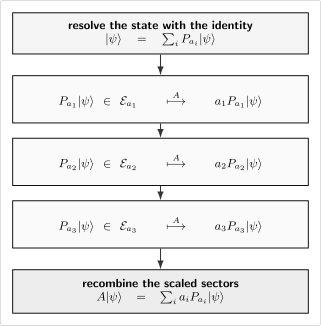
The identity resolves $|\psi\rangle$ into orthogonal components $P_{a_i}|\psi\rangle$. On each eigenspace, $A$ acts as multiplication by the corresponding value $a_i$.

Spectral Decomposition versus Diagonalization

Diagonalization is often written as

$$A=UDU^\dagger,$$

where $U$ is unitary and $D$ is diagonal. This is a matrix description after an orthonormal eigenbasis has been chosen. Spectral decomposition instead writes the basis-independent operator identity

$$A=\sum_a aP_a.$$

The distinction matters when an eigenvalue is degenerate:

• the diagonal matrix repeats the value once for each basis vector in its eigenspace;
• the spectral sum lists that value once and assigns it one higher-rank projector;
• a different orthonormal basis inside the degenerate eigenspace changes $U$ but leaves $P_a$ unchanged.

If $D$ has entries $a_1,\ldots,a_d$ and $|u_n\rangle$ are the columns of $U$, one may write

$$A = \sum_{n=1}^d a_n|u_n\rangle\langle u_n|.$$

When values repeat, this sum is over basis vectors rather than distinct outcomes. Grouping equal values recovers the spectral-projector form.

Nondegenerate Discrete Case

If each eigenvalue $a$ has a one-dimensional eigenspace and $|a\rangle$ is a normalized eigenvector, then

$$P_a = |a\rangle\langle a|.$$

The decomposition becomes

$$A = \sum_a a|a\rangle\langle a|,$$

with completeness relation

$$\sum_a|a\rangle\langle a|=I.$$

Acting on a state

$$|\psi\rangle = \sum_a c_a|a\rangle$$

gives

$$A|\psi\rangle = \sum_a a c_a|a\rangle.$$

This is the familiar textbook form. It is safe only when the sum is understood to include a complete eigenbasis and degeneracies are handled correctly.

Degenerate Discrete Case

Suppose the eigenspace $\mathcal E_a$ has dimension $g_a$. Choose any orthonormal basis

$$\left\lbrace |a,\lambda\rangle: \lambda=1,\ldots,g_a \right\rbrace.$$

The eigenspace projector is

$$P_a = \sum_{\lambda=1}^{g_a} |a,\lambda\rangle \langle a,\lambda|.$$

The spectral decomposition remains

$$A=\sum_a aP_a.$$

The index $a$ labels a distinct outcome; $\lambda$ labels basis vectors inside that outcome subspace. A unitary change of basis among the $|a,\lambda\rangle$ leaves $P_a$ invariant.

This is why a degenerate sharp measurement is specified by the full $P_a$, not by an arbitrary rank-one projector inside $\mathcal E_a$. The resulting state-update question is treated in Degenerate Measurements and Lüders Rule.

Uniqueness of the Spectral Projectors

For a self-adjoint $A$, the projector associated with a distinct eigenvalue is fixed by $A$ itself. It does not depend on a chosen eigenbasis.

In finite dimensions this can be seen through Lagrange interpolation. For each $a\in\sigma(A)$, define

$$q_a(x) = \prod_{\substack{b\in\sigma(A)\\b\neq a}} \frac{x-b}{a-b}.$$

This polynomial satisfies

$$q_a(b)=\delta_{ab}$$

on the spectrum. Applying it to $A$ gives

$$P_a = q_a(A) = \prod_{\substack{b\in\sigma(A)\\b\neq a}} \frac{A-bI}{a-b}.$$

On an eigenvector with value $c$, this product returns the vector if $c=a$ and zero otherwise. It therefore projects onto the entire $a$ eigenspace, including all degeneracy.

Two spectral values

If $A$ has exactly two distinct values $a$ and $b$, then

$$P_a = \frac{A-bI}{a-b}, \qquad P_b = \frac{A-aI}{b-a}.$$

These formulas extract the projectors without first writing eigenvectors. They are especially useful for qubits, parity sectors, and other binary observables.

Projector-Valued Decomposition

The phrase projector-valued decomposition emphasizes that the operator is not merely a list of eigenvalues. It is the pairing

$$a \longleftrightarrow P_a$$

between each distinct value and the subspace on which that value acts.

The values answer “what number is reported?” The projectors answer “which component of the state supports that outcome?” Both are needed to reconstruct $A$.

Two observables can have the same set of numerical eigenvalues but different projectors. For example, $\sigma_z$ and $\sigma_x$ both have values $\pm1$, but their eigenspaces differ. Their statistics in a given state therefore differ.

Conversely, assigning different distinct numerical labels to the same family of projectors changes the operator but keeps the same sharp partition of Hilbert space. This observation becomes precise under functions of operators and coarse graining below.

Decomposing a State into Outcome Sectors

For a normalized state, define

$$|\psi_a\rangle = P_a|\psi\rangle.$$

The sector components satisfy

$$\langle\psi_a|\psi_b\rangle=0 \qquad (a\neq b),$$

and

$$|\psi\rangle = \sum_a|\psi_a\rangle.$$

Their squared norms obey

$$\sum_a\|\psi_a\|^2=1.$$

When $\|\psi_a\|>0$, one may define the normalized sector vector

$$|\widehat\psi_a\rangle = \frac{P_a|\psi\rangle}{\|P_a\psi\|}.$$

Then

$$|\psi\rangle = \sum_{a:\,p(a)>0} \sqrt{p(a)} |\widehat\psi_a\rangle,$$

where the phase of each sector is inherited from $P_a|\psi\rangle$. This is an orthogonal decomposition of the original state, not yet a claim that a measurement has occurred.

Measurement Probabilities

For a normalized pure state, the Born probability of outcome $a$ is

$$p(a) = \langle\psi|P_a|\psi\rangle = \|P_a\psi\|^2.$$

Completeness guarantees normalization:

$$\begin{aligned} \sum_a p(a) &= \sum_a\langle\psi|P_a|\psi\rangle\\ &= \langle\psi|I|\psi\rangle\\ &=1. \end{aligned}$$

For a density operator $\rho$,

$$p(a) = \operatorname{Tr}(\rho P_a).$$

Spectral decomposition therefore separates the observable into the precise operators used to compute its outcome statistics. The canonical calculation workflow is Born Rule for Discrete Spectra.

Moments, Expectation Value, and Variance

Orthogonality of the spectral projectors gives

$$A^n = \sum_a a^nP_a$$

for every nonnegative integer $n$. Hence

$$\langle A^n\rangle_\psi = \sum_a a^n p(a).$$

In particular,

$$\langle A\rangle_\psi = \sum_a a p(a)$$

and

$$(\Delta A)^2 = \sum_a \left(a-\langle A\rangle_\psi\right)^2 p(a).$$

These are the ordinary moments and variance of the probability distribution induced by the state and the spectral projectors. Spectral decomposition does not replace the Born rule; it identifies the event operators to which the rule is applied.

Functions of an Observable

If $f$ is defined on the finite spectrum of $A$, then

$$f(A) = \sum_a f(a)P_a.$$

The eigenspaces remain the same while each value $a$ is replaced by $f(a)$. Examples include

$$\begin{aligned} A^2 &= \sum_a a^2P_a,\\ e^{-iAt} &= \sum_a e^{-iat}P_a,\\ |A| &= \sum_a |a|P_a. \end{aligned}$$

An inverse exists exactly when $0\notin\sigma(A)$, in which case

$$A^{-1} = \sum_a\frac{1}{a}P_a.$$

The full construction, including square roots, branch choices, and infinite-dimensional domains, is the canonical subject of Functions of Operators.

Relabeling and Coarse Graining

Suppose $B=f(A)$. Its values are $f(a)$, but distinct values of $a$ need not remain distinct.

If $f$ is one-to-one on $\sigma(A)$, then $A$ and $B$ have the same spectral projectors. They assign different numerical labels to the same sharp outcome subspaces.

If $f(a)=f(b)$ for two different values, the corresponding subspaces merge. For a value $\beta$ of $B$, its projector is

$$Q_\beta = \sum_{a:\,f(a)=\beta}P_a.$$

The observable $B$ is then a coarse graining of $A$: it cannot distinguish values that $f$ maps to the same label.

This distinction is physically useful. The operator $A^2$, for example, does not distinguish eigenvalues $a$ and $-a$ even when $A$ does.

Commuting Operators and Spectral Blocks

Let $A=\sum_a aP_a$ have distinct values $a$. For any operator $B$ in finite dimensions,

$$B = \sum_{a,b}P_aBP_b.$$

The terms $P_aBP_b$ are blocks mapping $\mathcal E_b$ into $\mathcal E_a$. The commutator is

$$[A,B] = \sum_{a,b} (a-b)P_aBP_b.$$

Therefore

$$[A,B]=0$$

if and only if all off-diagonal spectral blocks vanish:

$$P_aBP_b=0 \qquad (a\neq b).$$

Equivalently,

$$B = \sum_aP_aBP_a,$$

so $B$ preserves every eigenspace of $A$.

If $A$ is nondegenerate, each block is one-dimensional and a commuting self-adjoint $B$ is diagonal in the same eigenbasis. If $A$ is degenerate, $B$ can act nontrivially within each $\mathcal E_a$. Diagonalizing those restrictions is the first step toward a Complete Set of Commuting Observables.

Hamiltonians and Time Evolution

If a time-independent Hamiltonian has discrete spectral decomposition

$$H=\sum_E E P_E,$$

then

$$U(t) = e^{-iHt/\hbar} = \sum_E e^{-iEt/\hbar}P_E.$$

The evolved state is

$$|\psi(t)\rangle = \sum_E e^{-iEt/\hbar} P_E|\psi(0)\rangle.$$

Each energy sector acquires a phase. Every vector inside a degenerate energy eigenspace receives the same phase, so the state component within that eigenspace is not resolved further by $H$ alone.

The energy-sector weights are constant:

$$\|P_E\psi(t)\|^2 = \|P_E\psi(0)\|^2.$$

The dynamical interpretation is developed in Energy Eigenstates and Unitary Time Evolution.

Spectral Invariants

Let $g_a=\operatorname{rank}P_a$ be the degeneracy of $a$ in a finite-dimensional space. Spectral decomposition makes several basis-independent quantities immediate:

$$\begin{aligned} \operatorname{Tr}A &= \sum_a g_a a,\\ \det A &= \prod_a a^{g_a},\\ \|A\|_{\mathrm{op}} &= \max_a|a|. \end{aligned}$$

More generally,

$$\operatorname{Tr}f(A) = \sum_a g_a f(a).$$

The determinant formula includes multiplicity. It vanishes when zero is an eigenvalue, exactly when $A$ is not invertible.

Worked Example: A Two-Level Observable

Consider

$$A = \begin{pmatrix} 2&i\\ -i&2 \end{pmatrix}.$$

Its distinct eigenvalues are $1$ and $3$. Because there are only two values, the projectors can be extracted directly:

$$\begin{aligned} P_1 &= \frac{3I-A}{2} = \frac12 \begin{pmatrix} 1&-i\\ i&1 \end{pmatrix},\\ P_3 &= \frac{A-I}{2} = \frac12 \begin{pmatrix} 1&i\\ -i&1 \end{pmatrix}. \end{aligned}$$

They satisfy

$$P_1+P_3=I, \qquad P_1P_3=0,$$

and the reconstruction is

$$A=P_1+3P_3.$$

For the state $|0\rangle=(1,0)^{\mathsf T}$,

$$p(1) = \langle0|P_1|0\rangle = \frac12,$$

and similarly $p(3)=1/2$. Therefore

$$\langle A\rangle = 1\cdot\frac12 +3\cdot\frac12 =2,$$

which agrees with the direct matrix element $\langle0|A|0\rangle=2$.

Worked Example: Spin along an Axis

For a unit vector $\boldsymbol n$, define

$$\sigma_{\boldsymbol n} = \boldsymbol n\cdot\boldsymbol\sigma.$$

Its values are $+1$ and $-1$, with projectors

$$P_+ = \frac{I+\sigma_{\boldsymbol n}}{2}, \qquad P_- = \frac{I-\sigma_{\boldsymbol n}}{2}.$$

The spectral decomposition is

$$\sigma_{\boldsymbol n} = (+1)P_+ +(-1)P_- = P_+-P_-.$$

For spin angular momentum

$$S_{\boldsymbol n} = \frac{\hbar}{2} \sigma_{\boldsymbol n},$$

the projectors are unchanged while the values become $\pm\hbar/2$. The sharp alternatives are the same subspaces; only their numerical labels have been rescaled.

Continuous-Spectrum Form

For a self-adjoint operator with continuous or mixed spectrum, a simple sum of normalizable eigenprojectors is generally unavailable. The spectral theorem assigns a projection-valued measure $E_A$. The decomposition becomes the spectral integral

$$A = \int_{\mathbb R} \lambda\,dE_A(\lambda),$$

with identity resolution

$$I = E_A(\mathbb R) = \int_{\mathbb R}dE_A(\lambda).$$

For a Borel set $\Delta\subseteq\mathbb R$, the projector $E_A(\Delta)$ selects the spectral component whose values lie in $\Delta$. For a normalized pure state,

$$\Pr(A\in\Delta) = \langle\psi|E_A(\Delta)|\psi\rangle.$$

At a discrete eigenvalue,

$$E_A(\{a\})=P_a.$$

At a purely continuous spectral point, the singleton projector is typically zero even though every interval around the point has nonzero spectral projector. This is why the formal notation

$$A \sim \int a|a\rangle\langle a|\,da$$

is a useful heuristic but not the rigorous starting point: generalized kets $|a\rangle$ need not be Hilbert-space vectors.

Domain of an unbounded observable

If $A$ is unbounded, the spectral integral for $A$ is defined only on vectors whose second spectral moment is finite. Writing

$$\mu_\psi(\Delta) = \langle\psi|E_A(\Delta)|\psi\rangle,$$

the domain is

$$\mathcal D(A) = \left\lbrace |\psi\rangle: \int_{\mathbb R} \lambda^2\,d\mu_\psi(\lambda) <\infty \right\rbrace.$$

The projectors $E_A(\Delta)$ themselves are bounded and everywhere defined. This distinction lets spectral probabilities remain meaningful even when the state does not have a finite expectation value of $A^2$.

For point, continuous, essential, and mixed spectra, see Discrete and Continuous Spectra. For the rigorous working theorem, continue to Spectral Theorem, Practical Version.

What Self-Adjointness Contributes

In finite dimensions, every self-adjoint operator admits an orthogonal spectral decomposition with real values. More generally, every finite-dimensional normal operator has an orthogonal spectral decomposition, though its values may be complex.

A general nonnormal operator need not have an orthonormal eigenbasis. It may have nonorthogonal eigenvectors, oblique spectral projectors, or Jordan blocks. Writing an arbitrary matrix as if it had the observable decomposition

$$A=\sum_a aP_a$$

with mutually orthogonal $P_a$ is therefore unjustified.

For unbounded quantum observables, formal Hermiticity or symmetry on a test domain is not enough. The projection-valued spectral theorem requires a specified self-adjoint operator; see Hermitian vs Self-Adjoint Operators.

Practical Workflow

For a finite-dimensional self-adjoint observable:

1. Find the distinct eigenvalues. Keep track of their degeneracies.
2. Determine each eigenspace. Solve $(A-aI)|\psi\rangle=0$.
3. Construct $P_a$. Sum rank-one projectors over an orthonormal basis of the eigenspace, or use the polynomial formula.
4. Check orthogonality. Verify $P_aP_b=0$ for $a\neq b$.
5. Check completeness. Verify $\sum_aP_a=I$.
6. Reconstruct the operator. Verify $A=\sum_a aP_a$.
7. Compute statistics. Use $p(a)=\langle\psi|P_a|\psi\rangle$ or $p(a)=\operatorname{Tr}(\rho P_a)$.
8. Apply functions spectrally. Replace $a$ by $f(a)$ while keeping the projectors, then account for any merged values.

The completeness and reconstruction checks catch most missing-degeneracy and sign errors.

Common Mistakes

• Summing over eigenvectors without tracking repeated values. The basis-independent spectral sum is over distinct eigenvalues and full eigenspace projectors.
• Replacing a degenerate projector by one rank-one term. A sharp outcome $a$ corresponds to all of $\mathcal E_a$.
• Treating diagonalization as basis independent. The matrix $D$ and unitary $U$ depend on eigenbasis choices; the projectors $P_a$ do not.
• Applying $f$ to matrix entries. The rule is $f(A)=\sum_a f(a)P_a$, not entrywise evaluation in an arbitrary basis.
• Forgetting that a function can merge outcomes. If $f(a)=f(b)$, the spectral projector of $f(A)$ is $P_a+P_b$ for that combined value.
• Using eigenvalues without projectors to predict statistics. Equal spectra do not imply equal observables; the eigenspaces matter.
• Confusing state decomposition with measurement update. The identity $|\psi\rangle=\sum_aP_a|\psi\rangle$ is linear algebra, not a collapse postulate.
• Writing a continuous spectral integral as an ordinary sum of normalizable eigenstates. Use the projection-valued measure for the exact statement.
• Ignoring domains for unbounded operators. The spectral measure is everywhere defined, but $A$ and unbounded functions $f(A)$ are not.
• Applying the orthogonal formula to a nonnormal matrix. Nonnormal operators need not admit mutually orthogonal spectral projectors.

Scope and Canonical Boundaries

This page owns the physical reading of an observable as values paired with orthogonal outcome subspaces. Neighboring canonical pages carry the deeper pieces:

• Eigenvalues and Eigenstates develops eigenspaces, degeneracy, and definite values.
• Projectors develops subspace geometry and projector algebra.
• Mathematical Spectral Decomposition gives the finite-dimensional theorem as a linear-algebra tool.
• Functions of Operators develops the functional calculus and its domain restrictions.
• Born Rule for Discrete Spectra owns the measurement-probability workflow.
• Spectral Theorem, Practical Version owns projection-valued measures and spectral integrals in infinite dimensions.

Summary

• A finite-dimensional self-adjoint observable has the unique decomposition $A=\sum_a aP_a$ over its distinct eigenvalues.
• The projectors are mutually orthogonal and resolve the identity.
• Nondegenerate values give rank-one projectors; degenerate values give higher-rank eigenspace projectors.
• The formula is the basis-independent version of unitary diagonalization.
• Finite spectral projectors can be recovered as interpolation polynomials in $A$.
• A state decomposes into orthogonal sectors $P_a|\psi\rangle$, whose squared norms are Born probabilities.
• Moments, functions, and time evolution follow by applying the corresponding scalar expression to each spectral value.
• Commuting operators are block diagonal with respect to the spectral projectors.
• A non-injective function of $A$ coarse-grains its spectral outcomes.
• Continuous and mixed spectra replace the sum by $A=\int\lambda\,dE_A(\lambda)$.
• The projection-valued theorem requires self-adjointness and, for unbounded operators, explicit domain control.

References

• P. A. M. Dirac, The Principles of Quantum Mechanics, 4th ed., Oxford University Press, 1958.
• J. von Neumann, Mathematical Foundations of Quantum Mechanics, Princeton University Press, 1955.
• R. Shankar, Principles of Quantum Mechanics, 2nd ed., Springer, 1994.
• J. J. Sakurai and J. Napolitano, Modern Quantum Mechanics, 3rd ed., Cambridge University Press, 2020.
• B. C. Hall, Quantum Theory for Mathematicians, Springer, 2013.
• M. Reed and B. Simon, Methods of Modern Mathematical Physics, Volume I: Functional Analysis, Academic Press, 1980.
• S. Axler, Linear Algebra Done Right, 3rd ed., Springer, 2015.

Exercises

Exercise 1: Verify a two-level decomposition

For

$$A = \begin{pmatrix} 2&i\\ -i&2 \end{pmatrix},$$

verify directly that the matrices

$$P_1 = \frac12 \begin{pmatrix} 1&-i\\ i&1 \end{pmatrix}, \qquad P_3 = \frac12 \begin{pmatrix} 1&i\\ -i&1 \end{pmatrix}$$

are orthogonal projectors and reconstruct $A$.

Solution

Both matrices are self-adjoint. Direct multiplication gives

$$P_1^2=P_1, \qquad P_3^2=P_3, \qquad P_1P_3=0.$$

Their sum is

$$P_1+P_3=I.$$

Finally,

$$P_1+3P_3 = \begin{pmatrix} 2&i\\ -i&2 \end{pmatrix} =A.$$

Exercise 2: Projector interpolation

Let $A$ have distinct eigenvalues $-1$, $0$, and $2$. Write each spectral projector as a polynomial in $A$.

Solution

Using the interpolation formula,

$$\begin{aligned} P_{-1} &= \frac{A(A-2I)}{3},\\ P_0 &= -\frac{(A+I)(A-2I)}{2},\\ P_2 &= \frac{A(A+I)}{6}. \end{aligned}$$

Each polynomial equals one on its target value and zero on the other two. Consequently $P_{-1}+P_0+P_2=I$ on the whole Hilbert space.

Exercise 3: Degenerate outcome probabilities

Let

$$A = a \left( |1\rangle\langle1| +|2\rangle\langle2| \right) +b|3\rangle\langle3|,$$

where $a\neq b$, and let

$$|\psi\rangle = \frac{|1\rangle+i|2\rangle+\sqrt2|3\rangle}{2}.$$

Find the probabilities of $a$ and $b$ and the expectation value of $A$.

Solution

The spectral projectors are

$$P_a = |1\rangle\langle1| +|2\rangle\langle2|, \qquad P_b = |3\rangle\langle3|.$$

Therefore

$$p(a) = \frac14+\frac14 = \frac12, \qquad p(b) = \frac{2}{4} = \frac12.$$

The expectation value is

$$\langle A\rangle = \frac{a+b}{2}.$$

Exercise 4: Variance from spectral data

An observable has values $-2$, $0$, and $3$ with probabilities $1/4$, $1/2$, and $1/4$. Compute its expectation value and variance.

Solution

The expectation value is

$$\langle A\rangle = -2\left(\frac14\right) +3\left(\frac14\right) = \frac14.$$

The second moment is

$$\langle A^2\rangle = 4\left(\frac14\right) +9\left(\frac14\right) = \frac{13}{4}.$$

Hence

$$(\Delta A)^2 = \frac{13}{4} -\left(\frac14\right)^2 = \frac{51}{16}.$$

Exercise 5: Coarse graining by a function

Let

$$A = -2P_{-2} +P_1 +2P_2,$$

where the three projectors are mutually orthogonal and complete. Find the spectral decomposition of $A^2$.

Solution

Applying $f(a)=a^2$ gives

$$A^2 = 4P_{-2} +P_1 +4P_2.$$

The value $4$ occurs on two subspaces, so its spectral projector is their sum:

$$Q_4 = P_{-2}+P_2.$$

The distinct-value decomposition is therefore

$$A^2 = 1P_1 +4Q_4.$$

Squaring has erased the distinction between the values $-2$ and $2$.

Exercise 6: A commuting operator preserves eigenspaces

Let $A=\sum_a aP_a$ have distinct eigenvalues. Suppose $[A,B]=0$. Show that

$$P_aBP_b=0 \qquad (a\neq b).$$

Solution

Multiply the commutator by $P_a$ on the left and $P_b$ on the right:

$$\begin{aligned} 0 &= P_a[A,B]P_b\\ &= (a-b)P_aBP_b. \end{aligned}$$

For $a\neq b$, the scalar $a-b$ is nonzero, so $P_aBP_b=0$. Thus $B$ has no matrix blocks connecting different eigenspaces of $A$.

Exercise 7: Time evolution by energy sectors

Suppose

$$H=E_0P_0+E_1P_1, \qquad P_0+P_1=I.$$

Derive $U(t)$ and show that the probabilities of the two energy values are constant in time.

Solution

The spectral rule gives

$$U(t) = e^{-iE_0t/\hbar}P_0 +e^{-iE_1t/\hbar}P_1.$$

Because $P_jP_k=\delta_{jk}P_j$,

$$P_jU(t)|\psi(0)\rangle = e^{-iE_jt/\hbar} P_j|\psi(0)\rangle.$$

Taking the squared norm removes the phase:

$$\|P_j\psi(t)\|^2 = \|P_j\psi(0)\|^2.$$

Exercise 8: Continuous position projector

Let $X$ be the position operator on $L^2(\mathbb R)$ and let $R$ be a measurable region. The spectral projector acts as

$$\bigl(E_X(R)\psi\bigr)(x) = \mathbf1_R(x)\psi(x).$$

Verify the intersection rule

$$E_X(R)E_X(S) = E_X(R\cap S)$$

and identify the probability assigned to $R$.

Solution

Indicator functions obey

$$\mathbf1_R(x)\mathbf1_S(x) = \mathbf1_{R\cap S}(x).$$

Therefore multiplication by the first two indicators in succession equals multiplication by the indicator of the intersection. The Born probability is

$$\begin{aligned} \langle\psi|E_X(R)|\psi\rangle &= \int_{\mathbb R} \psi^*(x)\mathbf1_R(x)\psi(x)\,dx\\ &= \int_R|\psi(x)|^2\,dx. \end{aligned}$$