Operator Representations

An operator representation is a concrete coordinate form of an abstract operator. Depending on the chosen basis or representation map, the same operator can appear as a matrix, a multiplication rule, a differential expression, an integral kernel, or a diagonal spectral form.

The abstract operator is the basis-independent object. Its representative is the form used for a particular calculation. A valid change of representation must transform states, operators, inner products, and operator domains consistently.

This distinction is not cosmetic. It explains why momentum is a derivative in position space but a multiplier in momentum space, why a local potential becomes a momentum-mixing kernel, and why diagonal, sparse, or real-looking matrices are generally properties of a representation rather than of the operator itself.

The Representation Map

Let $A$ be an operator on a Hilbert space $\mathcal H$, with domain $D(A)$ when $A$ is unbounded. A representation $\mathcal R$ is implemented by a unitary map

$$\mathcal U_{\mathcal R}: \mathcal H\longrightarrow\mathcal K_{\mathcal R},$$

where $\mathcal K_{\mathcal R}$ is a coordinate Hilbert space such as $\mathbb C^n$, $\ell^2$, or $L^2(X,d\mu)$. Define

$$\begin{aligned} \psi_{\mathcal R} &=\mathcal U_{\mathcal R}\lvert\psi\rangle,\\ A_{\mathcal R} &=\mathcal U_{\mathcal R} A\mathcal U_{\mathcal R}^\dagger,\\ D(A_{\mathcal R}) &=\mathcal U_{\mathcal R}D(A). \end{aligned}$$

The represented action satisfies

$$A_{\mathcal R}\psi_{\mathcal R} = \mathcal U_{\mathcal R} A\lvert\psi\rangle.$$

This is the master translation rule. A matrix and a differential operator can represent the same $A$ because they act in different coordinate Hilbert spaces related by a unitary map.

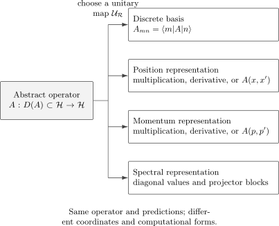
Each concrete form is obtained from the same abstract operator by a unitary representation map. Spectra, algebraic identities, and correctly paired predictions agree, while matrix entries and computational form can change.

From One Representation to Another

If $\mathcal R$ and $\mathcal S$ are two representations, the unitary map between their coordinate spaces is

$$W_{\mathcal S\mathcal R} = \mathcal U_{\mathcal S} \mathcal U_{\mathcal R}^\dagger.$$

Therefore

$$\begin{aligned} \psi_{\mathcal S} &=W_{\mathcal S\mathcal R} \psi_{\mathcal R},\\ A_{\mathcal S} &=W_{\mathcal S\mathcal R} A_{\mathcal R} W_{\mathcal S\mathcal R}^\dagger,\\ D(A_{\mathcal S}) &=W_{\mathcal S\mathcal R} D(A_{\mathcal R}). \end{aligned}$$

The detailed passive-basis convention and its alternatives are developed in Change of Basis. The practical rule is simple:

Never transform a state representative without transforming the operator representative and the inner product convention that go with it.

Predictions Are Representation Independent

Unitarity gives

$$\begin{aligned} \langle\phi\rvert A\lvert\psi\rangle &= \langle\phi_{\mathcal R}, A_{\mathcal R}\psi_{\mathcal R}\rangle_{\mathcal K_{\mathcal R}},\\ \lVert A\psi\rVert &= \lVert A_{\mathcal R}\psi_{\mathcal R}\rVert. \end{aligned}$$

Thus expectation values, transition amplitudes, and probabilities do not depend on the representation when every ingredient is translated consistently. This invariance is a useful error detector: two representations that give different predictions have not been matched correctly.

Discrete Orthonormal Bases

Let $\{\lvert e_n\rangle\}$ be a finite or countably infinite orthonormal basis. The state coordinates and operator matrix elements are

$$c_n=\langle e_n\vert\psi\rangle, \qquad A_{mn}=\langle e_m\rvert A\lvert e_n\rangle.$$

Using completeness, the represented action is matrix multiplication:

$$(A c)_m = \sum_n A_{mn}c_n.$$

In finite dimension, or with appropriate convergence in infinite dimension, the operator can be reconstructed as

$$A = \sum_{m,n} \lvert e_m\rangle A_{mn} \langle e_n\rvert.$$

This formula makes the distinction precise: $A$ is the map, while $[A_{mn}]$ is its coordinate array in the named basis. The underlying linear algebra is reviewed in Matrices as Linear Maps.

Matrix Algebra Mirrors Operator Algebra

In one orthonormal basis,

$$\begin{aligned} (AB)_{mn} &=\sum_k A_{mk}B_{kn},\\ (A^\dagger)_{mn} &=A_{nm}^*,\\ [A,B]_{mn} &=\sum_k \bigl(A_{mk}B_{kn}-B_{mk}A_{kn}\bigr). \end{aligned}$$

For a finite matrix, self-adjointness becomes $A_{mn}=A_{nm}^*$, and unitarity becomes $A^\dagger A=I$. These matrix conditions express invariant operator properties in a particular orthonormal basis.

In an infinite basis, formal matrix multiplication can hide convergence and domain issues. A column may lie outside $D(A)$ even when every individual matrix element is finite.

A Passive Basis Change

Let $S$ be the overlap matrix that sends old state components to new ones:

$$d=Sc.$$

With this convention, the operator matrix transforms as

$$A_{\mathrm{new}} = S A_{\mathrm{old}}S^\dagger.$$

The expectation value remains unchanged:

$$d^\dagger A_{\mathrm{new}}d = c^\dagger A_{\mathrm{old}}c.$$

Other books may define the overlap matrix in the opposite direction and write the inverse-looking conjugation. The physics agrees once the state and operator conventions are paired.

Generalized Continuous Representations

A continuous representation uses generalized kets $\{\lvert q\rangle\}$ satisfying a distributional completeness relation

$$\int_X \lvert q\rangle\langle q\rvert \,d\mu(q)=I.$$

The state representative is the wavefunction

$$\psi(q)=\langle q\vert\psi\rangle.$$

The generalized kets need not be normalizable vectors in $\mathcal H$. They are distributional tools whose precise setting is explained in Generalized Eigenvectors. The physical state remains the normalizable vector reconstructed from its wavefunction.

Operator Kernels Are Continuous Matrices

The continuous analogue of a matrix element is the kernel

$$A(q,q') = \langle q\rvert A\lvert q'\rangle.$$

It acts by

$$(A\psi)(q) = \int_X A(q,q')\psi(q') \,d\mu(q').$$

The analogy with matrix algebra is exact at the formal level:

$$\begin{aligned} (AB)(q,q') &=\int_X A(q,r)B(r,q') \,d\mu(r),\\ A^\dagger(q,q') &=A(q',q)^*. \end{aligned}$$

The identity kernel is the delta distribution appropriate to the measure:

$$I(q,q')=\delta_\mu(q,q').$$

Kernels need not be ordinary functions. Differential operators are represented by derivatives of delta distributions, and singular interactions may require additional distributional care.

Position Representation

For a particle on the line,

$$\psi(x)=\langle x\vert\psi\rangle.$$

The position and momentum operators act as

$$\begin{aligned} (Q\psi)(x)&=x\psi(x),\\ (P\psi)(x)&=-i\hbar\frac{d\psi}{dx}. \end{aligned}$$

For the common Hamiltonian

$$H=\frac{P^2}{2m}+V(Q),$$

the position representative is

$$(H\psi)(x) = \left[ -\frac{\hbar^2}{2m}\frac{d^2}{dx^2} +V(x) \right]\psi(x).$$

These differential expressions are incomplete without domains and boundary conditions. For example, the same formal derivative can describe different self-adjoint momentum operators on different configuration spaces.

Distributional Position Kernels

The preceding actions can be written as kernels:

$$\begin{aligned} Q(x,x') &=x\,\delta(x-x'),\\ P(x,x') &=-i\hbar\,\partial_x\delta(x-x'),\\ V(Q)(x,x') &=V(x)\delta(x-x'). \end{aligned}$$

For the Hamiltonian,

$$H(x,x') = \left[ -\frac{\hbar^2}{2m}\partial_x^2 +V(x) \right]\delta(x-x').$$

The derivative acts on the $x$ variable. After integration against $\psi(x')$, the delta distribution reproduces the familiar differential operator.

Momentum Representation

Choose the convention

$$\langle x\vert p\rangle = \frac{1}{\sqrt{2\pi\hbar}} e^{ipx/\hbar}.$$

The momentum-space wavefunction is $\phi(p)=\langle p\vert\psi\rangle$. In this representation,

$$\begin{aligned} (P\phi)(p)&=p\phi(p),\\ (Q\phi)(p)&=i\hbar\frac{d\phi}{dp}. \end{aligned}$$

The free Hamiltonian is a multiplication operator:

$$(H_0\phi)(p) = \frac{p^2}{2m}\phi(p).$$

The Fourier transform, normalization, and domain details are developed in Momentum-Space Representation.

A Local Potential Becomes Nonlocal in Momentum

Position-space multiplication by $V(x)$ has momentum-space kernel

$$\begin{aligned} V(p,p') &=\langle p\rvert V(Q)\lvert p'\rangle\\ &=\frac{1}{2\pi\hbar} \int_{\mathbb R} e^{-i(p-p')x/\hbar}V(x)\,dx. \end{aligned}$$

Therefore

$$(V\phi)(p) = \int_{\mathbb R} V(p,p')\phi(p')\,dp'.$$

A local potential generally mixes momenta. Conversely, a function of momentum is multiplicative in momentum space but generally nonlocal in position space. This is a concrete demonstration that computational locality depends on the chosen representation.

Spin Matrices

For spin $1/2$, choose the $S_z$ eigenbasis. Then

$$S_z = \frac{\hbar}{2} \begin{pmatrix} 1&0\\ 0&-1 \end{pmatrix},$$

while

$$S_x = \frac{\hbar}{2} \begin{pmatrix} 0&1\\ 1&0 \end{pmatrix}.$$

In the $S_x$ eigenbasis, $S_x$ is diagonal and $S_z$ is off-diagonal. Their eigenvalues and commutation relation do not change. The matrix pattern changes because the spin coordinate axes used for the components have changed.

The canonical matrix identities are collected in Pauli Matrices.

Energy and Spectral Representations

If $H$ has an orthonormal discrete energy eigenbasis,

$$H\lvert E_n\rangle=E_n\lvert E_n\rangle,$$

then

$$H_{mn}=E_n\delta_{mn}.$$

The Schrödinger equation reduces to independent component equations:

$$i\hbar\frac{dc_n}{dt}=E_nc_n,$$

with solution

$$c_n(t)=e^{-iE_nt/\hbar}c_n(0).$$

This simplicity is why the energy representation is adapted to a time-independent Hamiltonian. A different observable $A$ need not be diagonal in the same basis; its off-diagonal matrix elements connect energy sectors.

Degeneracy leaves freedom to rotate the basis inside an energy eigenspace. A complete set of commuting observables can supply additional labels. Continuous energy spectra require delta normalization and possible multiplicity labels rather than a simple list of normalizable vectors.

Worked Example: The Oscillator in Two Representations

For the one-dimensional harmonic oscillator, position representation gives

$$\begin{aligned} (Q\psi)(x)&=x\psi(x),\\ (H\psi)(x) &=\left[ -\frac{\hbar^2}{2m}\frac{d^2}{dx^2} +\frac12m\omega^2x^2 \right]\psi(x). \end{aligned}$$

In the number basis $\{\lvert n\rangle\}$, the Hamiltonian is diagonal:

$$H_{nm} = \hbar\omega \left(n+\frac12\right) \delta_{nm}.$$

Writing $q_0=\sqrt{\hbar/(2m\omega)}$, position is instead tridiagonal:

$$\begin{aligned} Q_{nm} &=q_0 \langle n\rvert(a+a^\dagger)\lvert m\rangle\\ &=q_0 \left[ \sqrt m\,\delta_{n,m-1} +\sqrt{m+1}\,\delta_{n,m+1} \right]. \end{aligned}$$

The multiplication operator and the infinite tridiagonal matrix are two exact representatives of the same abstract $Q$. Truncating the matrix to finitely many number states is a separate approximation.

Composite-System Representations

For a product basis

$$\lvert i,\alpha\rangle = \lvert i\rangle_A\otimes\lvert\alpha\rangle_B,$$

a local operator has matrix elements

$$(X_A\otimes I_B)_{i\alpha,j\beta} = (X_A)_{ij}\delta_{\alpha\beta}.$$

Changing local bases conjugates the matrix by $U_A\otimes U_B$. The abstract tensor-product operator and its locality to subsystem $A$ remain unchanged. The physical interpretation is developed in Subsystems and Local Observables.

Domains Transform with the Operator

For an unbounded operator, the pair $(A,D(A))$ is the operator. Under a unitary representation map,

$$D(A_{\mathcal R}) = \mathcal U_{\mathcal R}D(A).$$

This condition preserves self-adjointness:

$$A=A^\dagger \quad\Longleftrightarrow\quad A_{\mathcal R}=A_{\mathcal R}^\dagger,$$

where each adjoint is taken with its correct Hilbert-space inner product and domain.

A formal differential expression without a domain is not a complete representation of an unbounded operator. The canonical domain theory is in Domains of Operators and Hermitian vs Self-Adjoint Operators.

Active Transformations Are a Different Question

The conjugation $A\mapsto UAU^\dagger$ can appear in two conceptually distinct uses:

• A passive representation change rewrites the same state and operator in new coordinates. Predictions are unchanged because all representatives are transformed together.
• An active physical transformation changes the state, apparatus, or observable relative to a fixed coordinate description. It can represent a rotation, translation, symmetry operation, or time evolution.

The same matrix algebra can occur in both descriptions. One must state what is held fixed before assigning physical meaning.

Exact Representation Change versus Truncation

A unitary change of representation is exact and preserves the full operator. A finite truncation instead replaces $A$ by a compression such as

$$A^{(N)} = P_NAP_N \big\rvert_{P_N\mathcal H}.$$

This is generally not unitarily equivalent to $A$. It can change spectra, domains, commutators, and long-time dynamics. For example, finite matrices cannot satisfy the canonical commutator exactly because

$$\operatorname{Tr}[X,P]=0,$$

whereas

$$\operatorname{Tr}(i\hbar I_N) = i\hbar N.$$

Numerical basis calculations must therefore be checked for convergence as the truncation grows. The approximation strategy belongs to Discretization.

What Is Representation Invariant

Unitary equivalence preserves:

• the spectrum, including multiplicities and spectral type;
• self-adjointness, positivity, unitarity, and normality;
• operator norms and trace-class quantities when they are defined;
• products, adjoints, commutators, and functional identities;
• expectation values, transition amplitudes, and measurement probabilities;
• the dimension of kernels and spectral subspaces;
• the transformed domain structure of unbounded operators.

The following are generally representation dependent:

• state components and pointwise wavefunction values;
• individual matrix elements;
• whether a representative is diagonal, sparse, banded, real, or dense;
• whether an operator looks multiplicative, differential, or integral;
• which couplings appear as off-diagonal entries;
• the computational cost of applying the representative.

An invariant claim should survive unitary translation. A coordinate-dependent claim can still be useful, but its representation must be named.

Choosing a Useful Representation

• Position representation exposes local spatial potentials, geometry, boundary conditions, and configuration-space probability density.
• Momentum representation diagonalizes translations and free motion and turns derivatives into multipliers.
• Energy representation simplifies time evolution under a time-independent Hamiltonian.
• Spin or angular-momentum bases adapt calculations to a measurement axis or rotational symmetry.
• Symmetry-adapted bases block-diagonalize operators by conserved quantum numbers.
• Product bases expose subsystem structure and local operators.
• Numerical bases are chosen for sparsity, convergence, conditioning, and efficient matrix-vector products.

There is no universally best representation. The best one makes the dominant operator, symmetry, or boundary condition simple without obscuring the quantity being computed.

Practical Translation Audit

When comparing two operator formulas:

1. Identify the abstract Hilbert space and operator domain.
2. Name each basis or representation map and its measure convention.
3. Translate both the state and operator using the same unitary map.
4. Check whether generalized eigenkets and delta functions are being used distributionally.
5. Transform the domain and boundary conditions for unbounded operators.
6. Compare an invariant: a spectrum, matrix element, expectation value, commutator, or probability.
7. Distinguish exact unitary equivalence from projection, discretization, or truncation.
8. State whether the transformation is passive or an active physical operation.

For quick formula lookup after the conceptual audit, use the Representation Translation Table.

Common Mistakes

• Treating a matrix as the operator without naming its basis.
• Treating a differential expression as an operator without specifying its domain and boundary conditions.
• Transforming state components while leaving the operator in the old basis.
• Mixing overlap-matrix conventions from two sources.
• Assuming diagonal, sparse, local, or real-looking form is basis invariant.
• Treating generalized position or momentum kets as normalized Hilbert-space vectors.
• Forgetting the measure and Jacobian in a continuous completeness relation.
• Treating a derivative-of-delta kernel as an ordinary function.
• Confusing a passive rewrite with an active rotation or time evolution.
• Calling a finite basis truncation an exact change of representation.
• Assuming a degenerate eigenbasis is unique.
• Comparing individual matrix entries instead of invariant predictions.

Scope and Canonical Boundaries

This page is the canonical Core Formalism home for recognizing and translating the concrete forms of one operator.

• Bases and Representations owns state coordinates, basis completeness, and basis choice.
• Change of Basis derives overlap-matrix conventions, continuous transform kernels, and active versus passive distinctions in detail.
• Wavefunctions as Representations owns the interpretation of wavefunctions as state representatives.
• Momentum-Space Representation owns the position–momentum Fourier transform and momentum-space calculations.
• Spectral Decomposition owns diagonal spectral forms and projectors.
• Functions of Operators explains why operator functions transform consistently between representations.
• Coordinate Representation develops the wave-mechanics use of differential Hamiltonians.

Summary

• A representation is a unitary coordinate realization of an abstract operator.
• States, operators, inner products, and domains must be translated together.
• Discrete bases produce matrices; generalized continuous bases produce wavefunctions and kernels.
• Multiplication, differential, integral, and diagonal forms can represent the same operator.
• Spectra, algebraic identities, and physical predictions are invariant under exact unitary equivalence.
• Matrix entries, sparsity, diagonality, and computational locality generally depend on the chosen representation.
• A finite truncation is an approximation, not a representation change.

References

• P. A. M. Dirac, The Principles of Quantum Mechanics, 4th ed., Oxford University Press, 1958.
• J. von Neumann, Mathematical Foundations of Quantum Mechanics, Princeton University Press, 1955.
• R. Shankar, Principles of Quantum Mechanics, 2nd ed., Springer, 1994.
• J. J. Sakurai and J. Napolitano, Modern Quantum Mechanics, 3rd ed., Cambridge University Press, 2020.
• B. C. Hall, Quantum Theory for Mathematicians, Springer, 2013.
• M. Reed and B. Simon, Methods of Modern Mathematical Physics, Volume I: Functional Analysis, revised and enlarged ed., Academic Press, 1980.

Exercises

Exercise 1: Matrix action and reconstruction

Let $A_{mn}=\langle e_m\rvert A\lvert e_n\rangle$ in a finite orthonormal basis. Derive both

$$(Ac)_m=\sum_nA_{mn}c_n$$

and the reconstruction formula for $A$.

Solution

Insert completeness between the bra and the state:

$$\begin{aligned} \langle e_m\rvert A\lvert\psi\rangle &=\sum_n \langle e_m\rvert A\lvert e_n\rangle \langle e_n\vert\psi\rangle\\ &=\sum_nA_{mn}c_n. \end{aligned}$$

Insert completeness on both sides of $A$:

$$\begin{aligned} A &=IAI\\ &=\sum_{m,n} \lvert e_m\rangle \langle e_m\rvert A\lvert e_n\rangle \langle e_n\rvert\\ &=\sum_{m,n} \lvert e_m\rangle A_{mn}\langle e_n\rvert. \end{aligned}$$

Exercise 2: Spin basis change

In the $S_z$ basis, let

$$\sigma_z= \begin{pmatrix} 1&0\\ 0&-1 \end{pmatrix}, \qquad S=\frac{1}{\sqrt2} \begin{pmatrix} 1&1\\ 1&-1 \end{pmatrix}.$$

Compute $S\sigma_zS^\dagger$ and interpret the result.

Solution

The matrix $S$ is real, symmetric, and unitary. Direct multiplication gives

$$S\sigma_zS^\dagger = \begin{pmatrix} 0&1\\ 1&0 \end{pmatrix} = \sigma_x.$$

The old $z$-component operator is represented by $\sigma_x$ in the basis of $\sigma_x$ eigenvectors. Its eigenvalues remain $\pm1$; only its coordinate matrix has changed.

Exercise 3: Kernel product and adjoint

Starting from

$$(A\psi)(q) = \int A(q,r)\psi(r)\,d\mu(r),$$

derive the kernels of $AB$ and $A^\dagger$.

Solution

Apply $B$ first and substitute:

$$\begin{aligned} (AB\psi)(q) &=\int\!\!\int d\mu(r)\,d\mu(q')\\ &\qquad\times A(q,r)B(r,q')\psi(q'). \end{aligned}$$

Therefore

$$(AB)(q,q') = \int A(q,r)B(r,q')\,d\mu(r).$$

Comparing $\langle\phi,A\psi\rangle$ with $\langle A^\dagger\phi,\psi\rangle$ gives

$$A^\dagger(q,q')=A(q',q)^*.$$

Exercise 4: Canonical commutator in position space

On a common test domain, verify that $Q=x$ and $P=-i\hbar\,d/dx$ satisfy $[Q,P]\psi=i\hbar\psi$.

Solution

Compute the two orders:

$$\begin{aligned} (QP\psi)(x) &=-i\hbar x\psi'(x),\\ (PQ\psi)(x) &=-i\hbar\frac{d}{dx} \bigl(x\psi(x)\bigr)\\ &=-i\hbar\bigl(\psi(x)+x\psi'(x)\bigr). \end{aligned}$$

Subtracting gives

$$([Q,P]\psi)(x)=i\hbar\psi(x).$$

The calculation is valid on a domain where both compositions are defined. It does not by itself settle self-adjoint boundary conditions.

Exercise 5: Position in momentum space

Using

$$\phi(p) = \frac{1}{\sqrt{2\pi\hbar}} \int e^{-ipx/\hbar}\psi(x)\,dx,$$

show formally that multiplication by $x$ becomes $i\hbar\,d/dp$.

Solution

Let $c_\hbar=(2\pi\hbar)^{-1/2}$. Differentiating the transform gives

$$\phi'(p) = -\frac{i c_\hbar}{\hbar} \int x e^{-ipx/\hbar}\psi(x)\,dx.$$

Therefore

$$i\hbar\phi'(p) = c_\hbar \int e^{-ipx/\hbar}x\psi(x)\,dx.$$

The final expression is the Fourier transform of $Q\psi$. Hence

$$Q_p=i\hbar\frac{d}{dp}$$

on the transformed domain.

Exercise 6: Oscillator position matrix

Use

$$Q=q_0(a+a^\dagger), \qquad q_0=\sqrt{\frac{\hbar}{2m\omega}},$$

to show that the number-basis matrix of $Q$ is tridiagonal.

Solution

The ladder actions are

$$\begin{aligned} a\lvert m\rangle &=\sqrt m\lvert m-1\rangle,\\ a^\dagger\lvert m\rangle &=\sqrt{m+1}\lvert m+1\rangle. \end{aligned}$$

Therefore

$$\begin{aligned} Q_{nm} &=q_0\left[ \sqrt m\,\delta_{n,m-1} \right.\\ &\qquad\left. +\sqrt{m+1}\,\delta_{n,m+1} \right]. \end{aligned}$$

Only the first off-diagonals are nonzero, so the matrix is tridiagonal.

Exercise 7: Domain under Fourier transformation

Let $\mathcal F$ be the unitary position-to-momentum Fourier transform and let $P_x=-i\hbar\,d/dx$ be self-adjoint on its standard real-line domain. State the operator and domain of $P_p=\mathcal FP_x\mathcal F^\dagger$.

Solution

Fourier transformation turns differentiation into multiplication, so

$$(P_p\phi)(p)=p\phi(p).$$

The transformed domain is

$$D(P_p) = \left\{ \phi\in L^2(\mathbb R) \,\middle|\, p\phi\in L^2(\mathbb R) \right\}.$$

Equivalently, $D(P_p)=\mathcal F D(P_x)$. Carrying the domain through the unitary map is what preserves self-adjointness.

Exercise 8: Why truncation cannot preserve the canonical commutator

Show that no finite $N\times N$ matrices $X$ and $P$ can satisfy $[X,P]=i\hbar I_N$ exactly.

Solution

The trace of a finite matrix commutator vanishes by cyclicity:

$$\operatorname{Tr}[X,P] = \operatorname{Tr}(XP)-\operatorname{Tr}(PX) =0.$$

If $[X,P]=i\hbar I_N$, taking the trace would instead give

$$0=i\hbar\operatorname{Tr}I_N=i\hbar N,$$

which is impossible for $N>0$. A truncated basis can approximate canonical commutator matrix elements on well-resolved low-energy states, but it cannot be an exact finite-dimensional representation of the full canonical algebra.