Discrete and Continuous Spectra

The spectrum $\sigma(A)$ of an operator $A$ is the set of spectral values at which $A-\lambda I$ does not possess a suitably bounded, everywhere-defined inverse. For a finite-dimensional observable, the spectrum is exactly its set of eigenvalues. For an infinite-dimensional observable, the spectrum can also contain continuous values with no normalizable eigenvectors.

This distinction separates several familiar systems:

• a spin component has finitely many discrete outcomes;
• the harmonic oscillator has countably many discrete energy levels;
• position and momentum on the real line have continuous spectra;
• a finite potential well or Coulomb Hamiltonian has discrete bound-state energies and a scattering continuum.

The practical physics is encoded by spectral projectors. Discrete values carry projectors onto eigenspaces; intervals in a continuous spectrum carry projectors onto spectral bands. Probabilities are always assigned to measurable sets of outcomes, whether those sets contain isolated points, intervals, or both.

Spectrum of an Operator

Let $A$ be a closed operator on a complex Hilbert space. A complex number $z$ lies in the resolvent set $\rho(A)$ when

$$A-zI$$

is one-to-one, onto, and has a bounded inverse defined on the whole Hilbert space. The spectrum is the complement:

$$\sigma(A)=\mathbb C\setminus\rho(A).$$

For a self-adjoint operator,

$$\sigma(A)\subseteq\mathbb R,$$

as required for a real-valued sharp observable.

This definition may look more abstract than the eigenvalue equation, but it is the one that survives infinite dimension. In a $d$-dimensional space,

$$z\in\sigma(A) \quad\Longleftrightarrow\quad \det(A-zI)=0 \quad\Longleftrightarrow\quad A|\psi\rangle=z|\psi\rangle$$

for some nonzero $|\psi\rangle$. Thus every finite-dimensional spectral value is an eigenvalue.

Spectrum is an operator property

The spectrum depends on the operator, including its Hilbert space, domain, and boundary conditions. The same differential expression can have different spectra on the line, a finite interval, or a circle.

A normalized state does not change $\sigma(A)$. Instead, the state determines which parts of the spectrum receive nonzero probability. An observable can possess many spectral values that a particular state will never produce.

Spectrum, support, and one experiment

Three sets should not be conflated:

1. $\sigma(A)$ is the full spectrum allowed by the operator.
2. The support of the state’s spectral measure is the part that can occur with nonzero probability in that state.
3. One run returns one recorded value or finite-resolution bin.

For example, $\sigma(\sigma_z)=\{-1,+1\}$, but the state $|0\rangle$ assigns probability one to $+1$ and zero to $-1$.

Point Spectrum

The point spectrum consists of ordinary eigenvalues:

$$\sigma_{\mathrm p}(A) = \left\lbrace \lambda: \ker(A-\lambda I)\ne\{0\} \right\rbrace.$$

Each $\lambda\in\sigma_{\mathrm p}(A)$ has at least one normalizable eigenvector. For a self-adjoint observable, the associated eigenspace projector is

$$P_\lambda=P_A(\{\lambda\}),$$

and a normalized state has atomic probability

$$\Pr(A=\lambda) = \langle\psi|P_\lambda|\psi\rangle.$$

The point spectrum can be finite or infinite. The identity on an infinite-dimensional space has the single eigenvalue $1$ with infinite degeneracy. The harmonic oscillator has infinitely many nondegenerate eigenvalues accumulating only at infinity.

Discrete Spectrum

In operator theory, the discrete spectrum usually means isolated eigenvalues of finite multiplicity. In many physics texts, discrete spectrum is used more loosely for a finite or countable set of normalizable energy or observable eigenstates. The two uses agree for standard finite-dimensional, box-confined, and harmonic-oscillator examples, but they are not identical in full generality.

For a finite-dimensional Hermitian operator,

$$A=\sum_a aP_a,$$

and every spectral value is discrete. The Pauli operator

$$\sigma_z= \begin{pmatrix} 1&0\\ 0&-1 \end{pmatrix}$$

has

$$\sigma(\sigma_z)=\{-1,+1\}.$$

For the one-dimensional harmonic oscillator,

$$E_n = \hbar\omega \left(n+\frac12\right), \qquad n=0,1,2,\ldots,$$

so the energy spectrum is countably infinite and discrete. Therefore:

Discrete does not mean finite, and it does not mean finite-dimensional.

Degeneracy

A discrete eigenvalue can correspond to a multidimensional eigenspace. Its probability is computed with the whole eigenspace projector:

$$\Pr(A=a) = \langle\psi|P_a|\psi\rangle.$$

Choosing a basis $|a,\alpha\rangle$ inside that eigenspace gives

$$P_a = \sum_{\alpha=1}^{g_a} |a,\alpha\rangle\langle a,\alpha|,$$

but the projector is independent of that internal basis choice.

Accumulation and essential spectrum

An infinite list of eigenvalues can accumulate at a finite spectral value. That limit point is not an isolated discrete eigenvalue in the strict operator-theory sense. Eigenvalues of infinite multiplicity and finite accumulation points are typically counted as part of the essential spectrum.

This caveat rarely changes an elementary measurement calculation, but it matters when reading statements such as “the spectrum is purely discrete.” The intended convention should be stated.

Continuous Spectrum

A value $\lambda$ lies in the continuous spectrum when $A-\lambda I$ is one-to-one and has dense range, but its inverse is not bounded on that range. There is no nonzero normalizable vector satisfying

$$A|\psi\rangle=\lambda|\psi\rangle,$$

yet normalized states can be made increasingly concentrated near $\lambda$ in the spectral sense.

For self-adjoint operators, the point and continuous parts exhaust the spectrum in the standard residual-spectrum classification:

$$\sigma(A) = \sigma_{\mathrm p}(A) \cup \sigma_{\mathrm c}(A),$$

with no residual spectrum. More refined decompositions distinguish absolutely continuous and singular continuous parts. The standard position, momentum, and short-range scattering examples are absolutely continuous.

Approximate eigenstates

One way to recognize a spectral value is through a sequence of normalized vectors $|\psi_n\rangle$ such that

$$\|(A-\lambda I)|\psi_n\rangle\| \longrightarrow0.$$

For a self-adjoint operator, every spectral value admits such an approximate eigenvector sequence. At a point-spectrum value, the sequence can be constant at a true eigenvector. At a continuous-spectrum value, the sequence sharpens without converging to a normalizable exact eigenvector.

Broad wave packets centered around momentum $p_0$ in position space provide the physical picture: as their spatial width grows, their momentum spread shrinks, but the exact plane-wave limit leaves the Hilbert space.

Spectral Measures and Probabilities

The spectral theorem associates a projector $P_A(\Delta)$ with every suitable measurable set $\Delta\subseteq\mathbb R$. For a normalized pure state, define

$$\mu_\psi^A(\Delta) = \langle\psi|P_A(\Delta)|\psi\rangle.$$

This is a probability measure:

$$\mu_\psi^A(\mathbb R)=1, \qquad \mu_\psi^A(\Delta)\ge0.$$

If disjoint sets $\Delta_n$ are combined, their probabilities add:

$$\mu_\psi^A \left( \bigcup_n\Delta_n \right) = \sum_n \mu_\psi^A(\Delta_n).$$

This one formula covers every spectral type.

Atomic and continuous parts

For a discrete eigenvalue $a$,

$$\mu_\psi^A(\{a\}) = \langle\psi|P_a|\psi\rangle$$

can be nonzero. The measure has an atom at $a$.

For an absolutely continuous part, there is a density $w_\psi(\lambda)$ such that

$$\mu_\psi^A(\Delta) = \int_\Delta w_\psi(\lambda)\,d\lambda.$$

Then any single point has probability zero:

$$\mu_\psi^A(\{\lambda_0\})=0.$$

This does not mean $\lambda_0$ is impossible as a finite-precision readout. It means the ideal continuous probability measure assigns weight to intervals, not isolated points.

Mixed spectral measure

When the operator has both bound and continuum sectors, a state’s outcome measure can take the schematic form

$$\mu_\psi^H(dE) = \sum_n p_n\,\delta_{E_n}(dE) +w(E)\,dE.$$

The discrete probabilities and continuum density obey

$$\sum_n p_n +\int w(E)\,dE = 1.$$

This measure-level statement is safer than writing a bare “sum plus integral” resolution without specifying normalization and degeneracy conventions.

Generalized Eigenstates

Physicists represent a continuous spectral coordinate using formal kets $|\lambda,\alpha\rangle$:

$$A|\lambda,\alpha\rangle = \lambda|\lambda,\alpha\rangle.$$

The degeneracy or channel label $\alpha$ may be discrete or continuous. These kets generally do not lie in the Hilbert space. Their eigenvalue equation is understood weakly or distributionally.

With a simple absolutely continuous normalization,

$$\langle\lambda,\alpha |\lambda',\alpha'\rangle = \delta_{\alpha\alpha'} \delta(\lambda-\lambda').$$

The formal resolution of identity is

$$I = \sum_\alpha \int |\lambda,\alpha\rangle \langle\lambda,\alpha| \,d\lambda.$$

A normalizable state has spectral amplitudes

$$\psi_\alpha(\lambda) = \langle\lambda,\alpha|\psi\rangle$$

with

$$\sum_\alpha \int |\psi_\alpha(\lambda)|^2 \,d\lambda = 1.$$

The formal ket is not itself normalized to one. The square-integrable amplitude over the continuum defines the physical state.

Generalized kets are convention-dependent

Changing the spectral label changes the delta normalization. If $E=f(p)$, then

$$\delta\bigl(f(p)-E\bigr) = \sum_{p_i:\,f(p_i)=E} \frac{\delta(p-p_i)} {|f'(p_i)|},$$

with the sum accounting for all simple roots. Energy-normalized and momentum-normalized scattering kets therefore differ by square-root Jacobian factors, while probability densities differ by the full Jacobian. Degeneracy labels are essential when several momenta share the same energy.

This is why a density such as $|\psi(E)|^2$ depends on the chosen spectral coordinate even though probabilities for physical sets do not.

For the disciplined notation, see Generalized Eigenvectors. The distributional setting is Rigged Hilbert Spaces, First Look.

Position Spectrum on the Real Line

On $\mathcal H=L^2(\mathbb R)$, the position operator acts as

$$(X\psi)(x)=x\psi(x)$$

on its natural domain. Its spectrum is

$$\sigma(X)=\mathbb R,$$

and it has no normalizable eigenvectors. The formal generalized kets satisfy

$$X|x\rangle=x|x\rangle, \qquad \langle x|x'\rangle=\delta(x-x').$$

For a measurable region $\Delta$,

$$\bigl(P_X(\Delta)\psi\bigr)(x) = \mathbf 1_\Delta(x)\psi(x),$$

where $\mathbf 1_\Delta$ is the indicator function. Therefore,

$$\Pr(X\in\Delta) = \int_\Delta|\psi(x)|^2\,dx.$$

The projector onto a single point is zero in $L^2(\mathbb R)$:

$$P_X(\{x_0\})=0.$$

There is no normalized exact-position eigenstate even though every real $x_0$ is a spectral value.

Momentum Spectrum on the Real Line

For the standard self-adjoint momentum operator,

$$P=-i\hbar\frac{d}{dx},$$

the spectrum is also the full real line:

$$\sigma(P)=\mathbb R.$$

Its generalized position-space eigenfunctions are plane waves,

$$\langle x|p\rangle = \frac{1}{\sqrt{2\pi\hbar}} e^{ipx/\hbar},$$

with

$$\langle p|p'\rangle=\delta(p-p').$$

The constant modulus shows why a plane wave is not square-integrable:

$$\int_{\mathbb R} |\langle x|p\rangle|^2\,dx = \infty.$$

A normalizable state instead has momentum amplitude

$$\phi(p)=\langle p|\psi\rangle$$

and interval probabilities

$$\Pr(p_1\le P\le p_2) = \int_{p_1}^{p_2} |\phi(p)|^2\,dp.$$

See Momentum-Space Representation for the Fourier-transform conventions.

Boundary Conditions Can Discretize a Spectrum

The local differential formula does not determine the spectrum by itself. Configuration space and boundary conditions matter.

For a particle on a circle of circumference $L$, periodicity requires

$$\psi(x+L)=\psi(x).$$

Momentum eigenfunctions have the form $e^{ikx}$, and periodicity imposes

$$e^{ikL}=1.$$

Therefore,

$$k_n=\frac{2\pi n}{L}, \qquad p_n=\hbar k_n, \qquad n\in\mathbb Z.$$

Momentum is discrete on the circle but continuous on the line. The operator expression $-i\hbar\,d/dx$ is the same locally; the Hilbert space and domain are not.

The same lesson applies to energy. Confining boundary conditions can produce normalizable discrete levels, while open spatial directions support scattering continua.

Energy Spectra: Bound and Scattering States

For a time-independent Hamiltonian, spectral type reflects the qualitative motion permitted by the potential and boundary conditions.

Bound states

Bound-state eigenfunctions are normalizable and belong to the point spectrum:

$$H|E_n,\alpha\rangle = E_n|E_n,\alpha\rangle.$$

In standard confining one-dimensional problems, the discrete energy levels are isolated and accumulate only at infinity. In Coulomb systems, infinitely many negative bound-state energies accumulate at the continuum threshold.

Scattering states

Scattering states extend to spatial infinity and are usually generalized eigenvectors. For a free particle,

$$E=\frac{p^2}{2m},$$

so

$$\sigma(H) = [0,\infty).$$

In one spatial dimension, each $E>0$ corresponds to the two momentum channels

$$p=\pm\sqrt{2mE}.$$

Thus an energy label alone does not specify a unique generalized eigenstate.

Mixed spectra and thresholds

A finite attractive well commonly has negative discrete bound-state energies and a nonnegative continuum:

$$\sigma(H) = \{E_1,\ldots,E_N\} \cup [0,\infty),$$

when the potential is chosen to approach zero at infinity. The value $E=0$ is the continuum threshold under that convention.

The Coulomb Hamiltonian similarly has

$$E_n<0, \qquad E_n\longrightarrow0^-,$$

together with a scattering continuum $E\ge0$. The bound-state levels accumulate at the threshold, illustrating why “discrete” and “isolated from the entire spectrum by one common gap” are different claims.

See Free Particle, Finite Square Well, and Coulomb Continuum States: Overview for the canonical-system treatments.

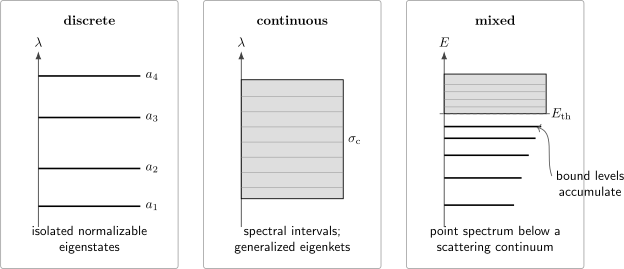
Three common spectral patterns. Isolated marks represent point-spectrum eigenvalues; the solid band represents a continuum. In a mixed Hamiltonian spectrum, bound levels can accumulate toward a scattering threshold.

Pure Point, Purely Continuous, and Mixed Spectra

The following physics terminology is useful:

• Pure point spectrum: the Hilbert space is spanned, in the relevant spectral sense, by normalizable eigenvectors. The harmonic oscillator is the standard example.
• Purely continuous spectrum: there are no normalizable eigenvectors in the spectral sector under discussion. Position and momentum on the line are standard examples.
• Mixed spectrum: point and continuous sectors both occur. Bound-plus- scattering Hamiltonians are standard examples.

These labels describe the operator’s spectral decomposition. A particular state may occupy only one sector. For example, a bound energy eigenstate of a mixed-spectrum Hamiltonian has no continuum probability until a physical interaction changes the state.

Finite Boxes and Continuum Limits

Calculations often place a system in a large box of length $L$ so that continuous momenta become discrete. With periodic boundary conditions,

$$p_n=\frac{2\pi\hbar n}{L}.$$

The spacing is

$$\Delta p=\frac{2\pi\hbar}{L}.$$

As $L\to\infty$,

$$\Delta p\longrightarrow0,$$

and sums are replaced by integrals:

$$\sum_n F(p_n) \;\longrightarrow\; \frac{L}{2\pi\hbar} \int_{\mathbb R}F(p)\,dp.$$

The factor $L/(2\pi\hbar)$ is a one-dimensional density of momentum states for this boundary convention. Correspondingly, box-normalized eigenvectors and delta-normalized generalized eigenvectors carry different normalization factors.

Finite-volume discretization is a regulator and computational device. It does not mean the infinite-volume continuum was secretly a finite list. One must take the limit with normalization and density-of-states factors consistently.

Expectations and Functions Across Spectral Types

The spectral measure unifies expectation values:

$$\langle A\rangle_\psi = \int_{\sigma(A)} \lambda\,d\mu_\psi^A(\lambda).$$

For a purely discrete measure, this reduces to

$$\langle A\rangle_\psi = \sum_a a\,p(a).$$

For a simple absolutely continuous representation,

$$\langle A\rangle_\psi = \int \lambda\,w_\psi(\lambda)\,d\lambda.$$

For a mixed measure, both terms appear. More generally,

$$\langle f(A)\rangle_\psi = \int_{\sigma(A)} f(\lambda)\,d\mu_\psi^A(\lambda),$$

provided the integral exists. This formula handles moments, unitary exponentials, and spectral filters without choosing a fictitious normalizable continuous eigenbasis.

Functions of Operators develops this calculus, including transformed outcome distributions and the domain test for unbounded $f(A)$.

Measurement Resolution and Binning

Real detectors report finite-resolution bins. If a detector associates an outcome label $j$ with a spectral set $\Delta_j$, the ideal coarse-grained probability is

$$p_j = \langle\psi|P_A(\Delta_j)|\psi\rangle.$$

For a continuous density,

$$p_j = \int_{\Delta_j} w_\psi(\lambda)\,d\lambda.$$

A histogram height depends on bin width; an integrated bin probability does not. This is one reason probability densities cannot be compared numerically to discrete probabilities without specifying units and resolution.

Finite resolution can also merge nearby discrete lines or blur a threshold. The mathematical spectrum, the apparatus response function, and the observed histogram are related but distinct.

Residual and Singular Continuous Spectra

The standard Core Formalism examples emphasize point and absolutely continuous spectra. Two additional terms appear in advanced work:

• The residual spectrum consists of values where $A-\lambda I$ is one-to-one but its range is not dense. A self-adjoint operator has no residual spectrum.
• A singular continuous spectrum is continuous and atom-free but supported on a set of Lebesgue measure zero. It appears in some quasiperiodic and fractal spectral problems.

These possibilities matter for operator theory and specialized quantum systems, but they should not be imported into every elementary position or scattering calculation. The canonical mathematical entry point is Continuous Spectra.

Rigorous Caveats

Several compact classroom formulas hide assumptions:

1. A self-adjoint operator may be unbounded, so its domain is part of its definition.
2. A continuous spectral value need not have any Hilbert-space eigenvector.
3. The notation $|\lambda\rangle$ can depend on the chosen spectral coordinate, degeneracy labels, and normalization measure.
4. A formal sum-plus-integral decomposition is justified by a direct-integral or spectral-measure construction, not by treating delta-normalized kets as ordinary vectors.
5. Embedded eigenvalues can occur inside a continuum in special systems, so a geometric drawing with levels only below threshold is an important example, not a universal theorem.
6. Resonances are generally not ordinary real eigenvalues of the self-adjoint Hamiltonian; they are identified through scattering or analytically continued resolvent structure.

The working theorem is Spectral Theorem, Practical Version. For domain precision, see Hermitian vs Self-Adjoint Operators.

A Practical Spectrum Audit

When a spectrum is quoted, ask:

1. Operator: What Hilbert space, domain, and boundary conditions define it?
2. Convention: Does “discrete” mean point spectrum or isolated finite-multiplicity eigenvalues?
3. Set: What is the actual spectral set $\sigma(A)$?
4. Type: Which parts are point, continuous, or mixed?
5. Eigenvectors: Which spectral values have normalizable eigenstates?
6. Degeneracy: What channel or quantum-number labels accompany each value?
7. Threshold: Where does a continuum begin, and what energy-zero convention is being used?
8. Measure: What is $P_A(\Delta)$ or the state-dependent $\mu_\psi^A(\Delta)$?
9. Density: With respect to which coordinate and measure is a probability density written?
10. Normalization: Are states normalized to one, a Kronecker delta, a Dirac delta, flux, or energy?
11. Resolution: Is the statement about the mathematical spectrum or a detector-broadened histogram?
12. Limit: If a box regulator is used, have the density-of-states factors been retained as volume tends to infinity?

Common Mistakes

• Equating spectrum with ordinary eigenvalues. This works in finite dimension but misses continuous spectral values.
• Saying every possible value has a normalizable eigenstate. Position, momentum, and scattering energy provide standard counterexamples.
• Treating “discrete” as synonymous with finite. A countably infinite spectrum can be discrete.
• Treating every point-spectrum eigenvalue as discrete in the strict sense. Infinite multiplicity or finite accumulation can place it in the essential spectrum.
• Treating a probability density as a probability. Densities have units and must be integrated over outcome sets.
• Assigning nonzero probability to one point in an absolutely continuous distribution. Singletons have measure zero.
• Reading $\delta(0)$ as a large finite norm. Delta normalization signals a generalized eigenvector, not a Hilbert-space unit vector.
• Dropping continuum degeneracy labels. Energy alone may not identify momentum direction, angular channel, spin, or scattering channel.
• Replacing sums by integrals without a density-of-states factor. Normalization changes in the continuum limit.
• Ignoring boundary conditions. Momentum is continuous on the line and discrete on a circle.
• Assuming bound states always exhaust the Hamiltonian. Many physical Hamiltonians also have scattering continua.
• Calling resonances bound-state eigenvalues. Resonant peaks and spectral eigenvalues are different objects.
• Confusing the operator’s spectrum with the support of one state’s outcome distribution.

Interpretation Boundary

The spectrum specifies the outcome space of an ideal sharp observable through its spectral measure. It does not by itself predict which outcomes are likely; that requires a state. Nor does it specify detector efficiency, resolution, line broadening, or the interaction by which the observable is measured.

Generalized eigenstates are coordinate tools for continuous spectral sectors. They need not be preparable exact states. A narrow wave packet can approximate a sharp continuous value over a finite range, but the ideal delta-normalized limit leaves the Hilbert space. Keeping the operator, state, spectral measure, and apparatus response distinct prevents both mathematical and interpretive overclaiming.

Summary

• In finite dimension, the spectrum is the set of eigenvalues.
• In infinite dimension, continuous spectral values can occur without normalizable eigenvectors.
• The point spectrum contains ordinary eigenvalues; the strict discrete spectrum contains isolated eigenvalues of finite multiplicity.
• Self-adjoint operators have real spectrum and no residual spectrum.
• Spectral projectors $P_A(\Delta)$ assign outcome sets to subspaces.
• A state defines the probability measure $\mu_\psi^A(\Delta)=\langle\psi|P_A(\Delta)|\psi\rangle$.
• Discrete probabilities are atoms; absolutely continuous probabilities are integrals of densities; mixed spectra contain both.
• Position and momentum on the line are continuous, while boundary conditions can discretize related operators.
• Bound-state energies belong to the point spectrum; scattering energies commonly form a continuum.
• Generalized eigenkets are distributional spectral coordinates, not finite-norm physical states.
• Box normalization approaches a continuum only with the correct density-of-states factors.

References

• P. A. M. Dirac, The Principles of Quantum Mechanics, 4th ed., Oxford University Press, 1958, Chapters II–III.
• J. von Neumann, Mathematical Foundations of Quantum Mechanics, Princeton University Press, 1955, Chapters II–III.
• R. Shankar, Principles of Quantum Mechanics, 2nd ed., Springer, 1994, Chapters 1 and 4.
• J. J. Sakurai and J. Napolitano, Modern Quantum Mechanics, 3rd ed., Cambridge University Press, 2020, Chapter 1.
• L. E. Ballentine, Quantum Mechanics: A Modern Development, World Scientific, 1998, Chapters 2–3.
• B. C. Hall, Quantum Theory for Mathematicians, Springer, 2013, Chapters 3–4 and 10.
• M. Reed and B. Simon, Methods of Modern Mathematical Physics, Volume I: Functional Analysis, revised and enlarged ed., Academic Press, 1980, Chapters VII–VIII.
• M. Reed and B. Simon, Methods of Modern Mathematical Physics, Volume III: Scattering Theory, Academic Press, 1979.
• G. Teschl, Mathematical Methods in Quantum Mechanics, 2nd ed., American Mathematical Society, 2014, Chapters 2–3.

Exercises

Exercise 1: Classify standard spectra

Classify each standard model as discrete, continuous, or mixed:

1. $\sigma_z$ on $\mathbb C^2$;
2. the harmonic oscillator Hamiltonian on the line;
3. momentum on the real line;
4. a finite attractive square well with negative bound states and continuum threshold at zero.

Solution

The classifications are:

1. $\sigma_z$ has the finite discrete spectrum $\{-1,+1\}$.
2. The harmonic oscillator has a countably infinite discrete spectrum $E_n=\hbar\omega(n+1/2)$.
3. Momentum on the line has continuous spectrum $\mathbb R$ and no normalizable momentum eigenvectors.
4. The finite attractive well has mixed spectrum: finitely many negative discrete bound-state energies and a continuum $[0,\infty)$ under the stated energy convention.

Exercise 2: Spectrum versus state support

Let $\sigma_z$ act on a qubit prepared in $|0\rangle$. State the full spectrum, the support of the state’s spectral measure, and the result distribution.

Solution

The operator spectrum is

$$\sigma(\sigma_z)=\{-1,+1\}.$$

Because $|0\rangle$ is the $+1$ eigenstate,

$$\Pr(+1)=1, \qquad \Pr(-1)=0.$$

The support of this state’s spectral measure is therefore the singleton $\{+1\}$, even though the operator itself also permits $-1$ in other states.

Exercise 3: Exact values in a continuum

Let $\phi(p)$ be a normalized momentum-space wavefunction. Explain why $\Pr(P=p_0)=0$ for an absolutely continuous distribution, and write the probability for a detector bin $[p_0-\Delta p/2,p_0+\Delta p/2]$.

Solution

A singleton has zero Lebesgue measure, so

$$\Pr(P=p_0) = \int_{\{p_0\}} |\phi(p)|^2\,dp = 0.$$

The finite-bin probability is

$$\Pr\left( p_0-\frac{\Delta p}{2} \le P\le p_0+\frac{\Delta p}{2} \right) = \int_{p_0-\Delta p/2}^{p_0+\Delta p/2} |\phi(p)|^2\,dp.$$

If the density varies slowly across a narrow bin, this is approximately $|\phi(p_0)|^2\Delta p$.

Exercise 4: Momentum on a circle

A wavefunction on a circle of circumference $L$ obeys $\psi(x+L)=\psi(x)$. Derive the allowed momenta for a plane wave $e^{ikx}$ and show that the spacing tends to zero as $L\to\infty$.

Solution

Periodicity requires

$$e^{ik(x+L)}=e^{ikx},$$

so

$$e^{ikL}=1.$$

Therefore

$$k_n=\frac{2\pi n}{L}, \qquad p_n=\frac{2\pi\hbar n}{L}, \qquad n\in\mathbb Z.$$

Adjacent momenta differ by

$$\Delta p=\frac{2\pi\hbar}{L}.$$

Hence $\Delta p\to0$ as $L\to\infty$, producing the continuum limit when normalizations and density-of-states factors are transformed consistently.

Exercise 5: Sum-to-integral conversion

For periodic boundary conditions in one dimension, use $p_n=2\pi\hbar n/L$ to derive

$$\sum_n F(p_n) \longrightarrow \frac{L}{2\pi\hbar} \int F(p)\,dp.$$

Solution

The momentum spacing is

$$\Delta p=\frac{2\pi\hbar}{L}.$$

A Riemann sum satisfies

$$\int F(p)\,dp \approx \sum_n F(p_n)\Delta p.$$

Solving for the sum gives

$$\sum_n F(p_n) \approx \frac{1}{\Delta p} \int F(p)\,dp = \frac{L}{2\pi\hbar} \int F(p)\,dp.$$

The prefactor is the density of allowed momentum values for this one- dimensional periodic box.

Exercise 6: Free-particle energy degeneracy

For a one-dimensional free particle,

$$E=\frac{p^2}{2m}.$$

For $E>0$, find the momentum branches and compute the Jacobian $|dp/dE|$. Explain why an energy-normalized basis needs a channel label.

Solution

The two momentum branches are

$$p_\pm(E)=\pm\sqrt{2mE}.$$

Differentiating,

$$\left|\frac{dp}{dE}\right| = \frac{m}{|p|} = \sqrt{\frac{m}{2E}}.$$

Both right-moving and left-moving generalized states share the same energy. An energy label $E$ alone therefore does not specify a unique state. One may use a discrete channel label such as $\alpha=+$ or $-$, together with the appropriate Jacobian factor when converting momentum normalization to energy normalization.

Exercise 7: A mixed probability measure

Suppose a Hamiltonian has one normalized bound state $|b\rangle$ with energy $E_b$ and a continuum $|E\rangle$. A normalized state is written formally as

$$|\psi\rangle = c_b|b\rangle +\int_0^\infty c(E)|E\rangle\,dE.$$

State the normalization condition and the probability that an energy measurement lies in $\{E_b\}\cup[E_1,E_2]$.

Solution

With the stated energy-delta normalization,

$$|c_b|^2 +\int_0^\infty |c(E)|^2\,dE = 1.$$

The discrete point and continuum interval are disjoint, so their probabilities add:

$$\Pr\left( H\in\{E_b\}\cup[E_1,E_2] \right) = |c_b|^2 +\int_{E_1}^{E_2} |c(E)|^2\,dE.$$

Exercise 8: Approximate eigenvectors

Let $X$ be the position operator on $L^2(\mathbb R)$. Construct a normalized sequence concentrated near $x_0$,

$$\psi_\epsilon(x) = \frac{1}{\sqrt{\epsilon}} f\left(\frac{x-x_0}{\epsilon}\right),$$

where $\int|f(u)|^2du=1$ and $f$ has finite second moment. Show that $\|(X-x_0I)\psi_\epsilon\|\to0$ as $\epsilon\to0$.

Solution

First, the substitution $u=(x-x_0)/\epsilon$ gives

$$\int|\psi_\epsilon(x)|^2\,dx = \int|f(u)|^2\,du = 1.$$

For the approximate eigenvalue error,

$$\begin{aligned} \|(X-x_0I)\psi_\epsilon\|^2 &= \int (x-x_0)^2 |\psi_\epsilon(x)|^2\,dx\\ &= \epsilon^2 \int u^2|f(u)|^2\,du. \end{aligned}$$

The integral is finite by assumption, so the squared norm is proportional to $\epsilon^2$ and tends to zero. The sequence becomes sharply localized around $x_0$, but its limiting delta distribution is not a vector in $L^2(\mathbb R)$.

Exercise 9: Density depends on coordinate

Let a positive momentum distribution be described by density $w_p(p)$ for $p>0$, and define energy $E=p^2/(2m)$. Derive the corresponding energy density $w_E(E)$ by requiring equal probabilities.

Solution

Probability is invariant under the coordinate change:

$$w_E(E)\,dE = w_p(p)\,dp.$$

For $p=\sqrt{2mE}$,

$$\frac{dp}{dE} = \frac{m}{p} = \sqrt{\frac{m}{2E}}.$$

Therefore,

$$w_E(E) = w_p\left(\sqrt{2mE}\right) \sqrt{\frac{m}{2E}}.$$

The numerical density changes because its units and reference measure change; integrated probabilities do not.