Functions of Operators

A function of an operator is obtained by applying a scalar function to the operator’s spectral values while retaining its spectral subspaces. It is not, in general, obtained by applying the function separately to the entries of one matrix representation.

For a self-adjoint operator with finite spectral decomposition

$$A=\sum_j a_jP_j,$$

the defining rule is

$$f(A)=\sum_j f(a_j)P_j.$$

This one construction gives precise meanings to $A^2$, $\sqrt A$, $A^{-1}$, $e^{-iHt/\hbar}$, spectral projectors, and many other expressions used throughout quantum mechanics. When $f$ is real-valued, it also has a direct physical interpretation: measuring $f(A)$ amounts to measuring $A$ and reporting the transformed outcome $f(a)$.

Scope and Conventions

The main object on this page is a self-adjoint operator $A$. Finite-dimensional operators come first because all domain questions disappear and the essential idea is visible in a finite sum. The later sections state the corresponding spectral-integral construction for continuous spectra and unbounded functions.

Three conventions matter:

• $\sigma(A)$ denotes the spectrum of $A$.
• A scalar function only needs to be specified on $\sigma(A)$; changing it away from the spectrum does not change $f(A)$.
• When $f$ is unbounded, the domain $D(f(A))$ is part of the definition.

General functions of nonnormal or nondiagonalizable matrices require additional machinery. Their finite-dimensional construction belongs to Matrix Functions and Exponentials.

Finite-Dimensional Spectral Definition

Let $A=A^\dagger$ act on a finite-dimensional Hilbert space. Write its spectral decomposition using the distinct eigenvalues $a_1,\ldots,a_r$:

$$\begin{aligned} A&=\sum_{j=1}^{r}a_jP_j,\\ P_jP_k&=\delta_{jk}P_j,\\ \sum_{j=1}^{r}P_j&=I. \end{aligned}$$

For any function $f$ defined on the finite set $\sigma(A)$, define

$$f(A)=\sum_{j=1}^{r}f(a_j)P_j.$$

If $\lvert a_j,\alpha\rangle$ belongs to the eigenspace $P_j\mathcal H$, then

$$f(A)\lvert a_j,\alpha\rangle = f(a_j)\lvert a_j,\alpha\rangle.$$

The degeneracy label $\alpha$ is untouched. Functional calculus changes the spectral value attached to an eigenspace, not the vectors inside that eigenspace.

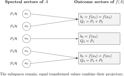
Functional calculus retains each subspace $P_j\mathcal H$ while replacing $a_j$ by $f(a_j)$. If several values have the same image $b$, the corresponding spectral projector of $f(A)$ is their sum, such as $Q_1=P_1+P_2$.

Basis Independence

Suppose $A$ is diagonalized as

$$A=UDU^\dagger, \qquad D=\operatorname{diag}(a_1,\ldots,a_n).$$

Then

$$f(A)=Uf(D)U^\dagger,$$

where

$$f(D)=\operatorname{diag} \bigl(f(a_1),\ldots,f(a_n)\bigr).$$

More generally, under a unitary change of representation,

$$A'=VAV^\dagger \quad\Longrightarrow\quad f(A')=Vf(A)V^\dagger.$$

This covariance is the test that an operator construction is independent of a chosen basis.

Why entrywise substitution fails

Consider

$$A= \begin{pmatrix} 1&1\\ 1&1 \end{pmatrix}.$$

Applying $x\mapsto x^2$ to each entry leaves this matrix unchanged. The operator square instead means composition:

$$A^2=AA = \begin{pmatrix} 2&2\\ 2&2 \end{pmatrix}.$$

Entrywise substitution depends on the displayed basis and usually does not represent any intrinsic function of the operator.

Algebraic Laws

For finite-dimensional $A$, or for bounded functions in the general spectral calculus, the map $f\mapsto f(A)$ preserves the ordinary algebra of scalar functions. For scalars $\alpha,\beta$,

$$\begin{aligned} 1(A)&=I,\\ \operatorname{id}(A)&=A,\\ (\alpha f+\beta g)(A) &=\alpha f(A)+\beta g(A),\\ (fg)(A)&=f(A)g(A),\\ \overline f(A)&=f(A)^\dagger,\\ (g\circ f)(A)&=g\bigl(f(A)\bigr). \end{aligned}$$

The product law follows immediately from orthogonality of the spectral projectors:

$$\begin{aligned} f(A)g(A) &= \sum_{j,k}f(a_j)g(a_k)P_jP_k\\ &= \sum_j f(a_j)g(a_j)P_j\\ &=(fg)(A). \end{aligned}$$

Several useful tests follow:

• If $f$ is real-valued on $\sigma(A)$, then $f(A)$ is self-adjoint.
• If $f(a)\geq0$ on $\sigma(A)$, then $f(A)$ is positive.
• If $\lvert f(a)\rvert=1$ on $\sigma(A)$, then $f(A)$ is unitary.
• Every $f(A)$ commutes with $A$ and with every spectral projector $P_j$.

For unbounded $f$ and $g$, these formulas acquire domain qualifications. One must not replace operator inclusions by equalities without checking the domains of the sums and products.

Spectrum, Norm, and Kernel

In finite dimensions, the spectral mapping rule is exact:

$$\sigma\bigl(f(A)\bigr)=f\bigl(\sigma(A)\bigr).$$

Repeated values are listed only once in the set on the right. The operator norm and kernel are

$$\lVert f(A)\rVert = \max_{a\in\sigma(A)}\lvert f(a)\rvert,$$

and

$$\ker f(A) = \bigoplus_{a:\,f(a)=0}P_a\mathcal H.$$

For a bounded self-adjoint operator and continuous $f$, the same spectral mapping and norm formulas hold, with the maximum taken over the compact spectrum. For a merely Borel function, the correct general statement uses its essential range relative to the projection-valued spectral measure; the naive set-theoretic image can contain values carried by no spectral weight.

Relabeling and Coarse Graining

Let $b$ be a distinct value of $f$ on $\sigma(A)$. The spectral projector of $f(A)$ associated with $b$ is

$$Q_b = \sum_{a:\,f(a)=b}P_a.$$

There are two qualitatively different cases.

Injective functions preserve all spectral labels

If $f$ is one-to-one on $\sigma(A)$, every $a$ can be recovered from $b=f(a)$. The observables $A$ and $f(A)$ have the same spectral projectors, and there is a function $h$ on $f(\sigma(A))$ such that

$$h\bigl(f(A)\bigr)=A.$$

Thus $f(A)$ contains exactly the same sharp spectral information as $A$.

Noninjective functions merge outcomes

If $f(a_j)=f(a_k)$ for distinct eigenvalues, $f(A)$ cannot distinguish the corresponding eigenspaces. Their projectors add. This is a genuine coarse graining of the sharp observable, even though the operator remains a perfectly well-defined function of $A$.

This distinction is central when deciding whether a derived operator supplies a new label in a complete set of commuting observables. A function of one member automatically commutes with it, but it may be redundant or may erase labels rather than resolve them.

Measurement Distribution of a Function

In this section, let $f$ be real-valued on $\sigma(A)$, so $f(A)$ is again a self-adjoint observable. Let $P^A(\Delta)$ be the spectral projector of $A$ for a Borel set $\Delta\subseteq\mathbb R$. The projection-valued measure of $f(A)$ obeys

$$P^{f(A)}(\Delta) = P^A\bigl(f^{-1}(\Delta)\bigr).$$

For a state $\rho$, define the outcome measure

$$\mu_\rho^A(\Delta) = \operatorname{Tr}\!\left[ \rho P^A(\Delta) \right].$$

Then

$$\mu_\rho^{f(A)}(\Delta) = \mu_\rho^A\bigl(f^{-1}(\Delta)\bigr).$$

In probability language, the distribution of $f(A)$ is the pushforward of the distribution of $A$ under $f$. In the finite discrete case,

$$\Pr\bigl(f(A)=b\bigr) = \sum_{a:\,f(a)=b}\Pr(A=a).$$

Whenever the expectation is defined,

$$\langle f(A)\rangle_\rho = \int_{\sigma(A)}f(\lambda) \,d\mu_\rho^A(\lambda).$$

Powers give moments, so $\langle A^2\rangle$ and the variance are special cases of this rule. Their statistical interpretation is developed in Variance and Standard Deviation.

Which Commuting Operators Are Functions?

Every $f(A)$ commutes with $A$, but the converse depends on degeneracy.

If $A$ has a nondegenerate finite spectrum, every operator $B$ satisfying $[A,B]=0$ is diagonal in the eigenbasis of $A$. Assigning the corresponding diagonal value of $B$ to each eigenvalue of $A$ defines a function $f$ such that

$$B=f(A).$$

If $A$ has degenerate eigenspaces, an operator commuting with $A$ may act nontrivially inside each eigenspace. A function $f(A)$ cannot do that: it is a scalar multiple of the identity on every $P_a\mathcal H$. Therefore

$$\bigl\{f(A)\bigr\} \subsetneq \bigl\{B:[A,B]=0\bigr\}$$

in a typical degenerate case.

This is the operator-algebra version of the statement that a single degenerate observable does not label a basis completely.

Every Finite Spectral Function Is a Polynomial

Although $f$ may be nonanalytic or even discontinuous away from the spectrum, its values on a finite spectrum can always be interpolated by a polynomial. Define

$$\ell_j(x) = \prod_{k\ne j} \frac{x-a_k}{a_j-a_k}.$$

These polynomials satisfy $\ell_j(a_k)=\delta_{jk}$ and

$$P_j=\ell_j(A).$$

Consequently,

$$f(A) = \sum_{j=1}^{r}f(a_j)\ell_j(A).$$

Thus every function of a finite-dimensional self-adjoint operator equals a polynomial in that operator of degree at most $r-1$. This statement concerns agreement on the finite spectral set; it does not claim that the original scalar function is globally polynomial.

Polynomial and Power-Series Routes

For a polynomial

$$p(x)=\sum_{n=0}^{N}c_nx^n,$$

the spectral definition agrees with ordinary operator algebra:

$$p(A)=\sum_{n=0}^{N}c_nA^n.$$

If a power series for $f$ converges uniformly on the spectrum, then the same series may be applied to $A$:

$$f(A)=\sum_{n=0}^{\infty}c_nA^n.$$

The spectral rule is more general. It defines discontinuous functions such as characteristic functions and sign functions, for which no globally convergent Taylor series is available. A series is therefore a computational route under appropriate convergence conditions, not the universal definition.

Positive Square Roots and Absolute Values

Let $B$ be a positive self-adjoint operator. Since its spectrum is contained in $[0,\infty)$, the nonnegative square-root function defines

$$B^{1/2} = \int_{\sigma(B)}\sqrt{\lambda} \,dP^B(\lambda).$$

In finite dimensions this is

$$B^{1/2}=\sum_j\sqrt{b_j}\,P_j.$$

It is the unique positive self-adjoint operator satisfying

$$\bigl(B^{1/2}\bigr)^2=B.$$

The adjective positive removes the branch ambiguity. An operator can have other square roots, and a scalar square-root branch need not be defined on the spectrum of a general operator.

For self-adjoint $A$, its absolute value is

$$\lvert A\rvert = \bigl(A^2\bigr)^{1/2} = \int_{\sigma(A)}\lvert\lambda\rvert \,dP^A(\lambda).$$

Defining $\operatorname{sgn}(0)=0$ gives the bounded sign operator and the factorization

$$A=\operatorname{sgn}(A)\lvert A\rvert$$

on $D(A)$. This is the self-adjoint case of polar decomposition.

Inverses, Reciprocals, and Zero

For a finite-dimensional operator,

$$A^{-1} = \sum_j\frac{1}{a_j}P_j$$

exists exactly when no eigenvalue is zero. For a general self-adjoint operator, the bounded everywhere-defined inverse exists exactly when

$$0\notin\sigma(A).$$

The distinction between spectrum and point spectrum now matters. It is possible that $0\in\sigma(A)$ even though $0$ is not an eigenvalue. In that case the reciprocal function may define a densely defined, unbounded inverse:

$$A^{-1} = \int_{\sigma(A)}\frac{1}{\lambda} \,dP^A(\lambda),$$

with a proper domain determined by square integrability near $\lambda=0$. The scalar function may be assigned any finite value at $\lambda=0$ because the spectral projector of that singleton vanishes in this case.

If zero is an eigenvalue, no two-sided inverse exists on the full Hilbert space. The Moore–Penrose pseudoinverse instead uses

$$f(\lambda) = \begin{cases} 1/\lambda,&\lambda\ne0,\\ 0,&\lambda=0. \end{cases}$$

It annihilates the kernel. In infinite dimensions it can still be unbounded if nonzero spectral values accumulate at zero.

Exponentials and Unitary Groups

For self-adjoint $A$ and real $s$, the function $e^{-is\lambda}$ has unit modulus. Therefore

$$e^{-isA} = \int_{\sigma(A)}e^{-is\lambda} \,dP^A(\lambda)$$

is a bounded unitary operator on the whole Hilbert space, even when $A$ itself is unbounded. It satisfies

$$\begin{aligned} e^{-isA}e^{-itA}&=e^{-i(s+t)A},\\ \bigl(e^{-isA}\bigr)^\dagger&=e^{isA}. \end{aligned}$$

For a time-independent self-adjoint Hamiltonian,

$$U(t)=e^{-iHt/\hbar}.$$

Each energy sector acquires the phase $e^{-iEt/\hbar}$. The dynamical meaning, continuity in $t$, and generator relation belong to Unitary Time Evolution.

By contrast, $e^{sA}$ for real $s$ need not be bounded when $A$ is unbounded. Its domain must then be determined from the spectral growth of $e^{s\lambda}$.

A Useful Projector Identity

An orthogonal projector $P$ has spectrum contained in $\{0,1\}$. Hence

$$f(P)=f(0)(I-P)+f(1)P.$$

For the exponential,

$$e^{\alpha P} = I+\bigl(e^\alpha-1\bigr)P.$$

This identity is often faster than expanding the series. It follows equally from $P^n=P$ for every $n\geq1$.

The Resolvent as a Function

For $z\notin\sigma(A)$, the scalar function

$$f_z(\lambda)=\frac{1}{z-\lambda}$$

is bounded on the spectrum. It defines the resolvent

$$\begin{aligned} R_A(z)&=(zI-A)^{-1}\\ &=\int_{\sigma(A)} \frac{1}{z-\lambda} \,dP^A(\lambda). \end{aligned}$$

For self-adjoint $A$,

$$\lVert R_A(z)\rVert = \frac{1}{\operatorname{dist} \bigl(z,\sigma(A)\bigr)}.$$

The resolvent packages spectral and dynamical information, but its analytic structure and boundary values have their canonical treatment in Resolvent Operator.

Worked Example: Squaring Spin One

Let $J_z$ act in the spin-one space, with projectors $P_+$, $P_0$, and $P_-$:

$$J_z = \hbar P_+-\hbar P_-.$$

Applying $f(m\hbar)=m^2\hbar^2$ gives

$$J_z^2 = \hbar^2(P_++P_-).$$

The outcomes of $J_z^2$ are $0$ and $\hbar^2$. For

$$\lvert\psi\rangle = c_+\lvert+1\rangle +c_0\lvert0\rangle +c_-\lvert-1\rangle,$$

their probabilities are

$$\begin{aligned} \Pr(J_z^2=0)&=\lvert c_0\rvert^2,\\ \Pr(J_z^2=\hbar^2) &=\lvert c_+\rvert^2+\lvert c_-\rvert^2. \end{aligned}$$

Squaring has merged the $m=+1$ and $m=-1$ sectors. Measuring $J_z^2$ cannot recover the sign of the original $J_z$ outcome.

Worked Example: Any Function of a Qubit Observable

Write a Hermitian two-level operator as

$$A=a_0I+\mathbf a\cdot\boldsymbol\sigma.$$

For $r=\lVert\mathbf a\rVert>0$, define

$$N=\widehat{\mathbf a}\cdot\boldsymbol\sigma, \qquad N^2=I.$$

The two eigenvalues and projectors are

$$a_\pm=a_0\pm r, \qquad P_\pm=\frac{I\pm N}{2}.$$

Therefore every function of $A$ reduces to

$$\begin{aligned} f(A) &=f(a_+)P_++f(a_-)P_-\\ &= \frac{f(a_+)+f(a_-)}{2}I\\ &\quad+ \frac{f(a_+)-f(a_-)}{2}N. \end{aligned}$$

Choosing $f(x)=e^{-isx}$ yields

$$e^{-isA} = e^{-isa_0} \left[ \cos(sr)I-i\sin(sr)N \right].$$

This is the spectral origin of the familiar Pauli-matrix exponential. If $r=0$, then $A=a_0I$ and simply $f(A)=f(a_0)I$.

Continuous Spectra and Spectral Integrals

For a self-adjoint operator with projection-valued measure $P^A$, the general definition is

$$f(A) = \int_{\sigma(A)}f(\lambda) \,dP^A(\lambda).$$

This includes discrete, continuous, and mixed spectra in one expression. A bounded Borel function gives a bounded normal operator on all of $\mathcal H$. If $f$ is real-valued, $f(A)$ is self-adjoint; if $f\geq0$, it is positive.

The construction and the projection-valued measure are developed from the mathematical side in Spectral Theorem, Practical Version.

Natural Domain of an Unbounded Function

For $\lvert\psi\rangle\in\mathcal H$, define its scalar spectral measure by

$$\mu_\psi^A(\Delta) = \langle\psi\rvert P^A(\Delta) \lvert\psi\rangle.$$

If $f$ is unbounded, a vector $\psi$ belongs to $D(f(A))$ exactly when

$$\int_{\sigma(A)} \lvert f(\lambda)\rvert^2 \,d\mu_\psi^A(\lambda)<\infty.$$

On this domain,

$$\lVert f(A)\psi\rVert^2 = \int_{\sigma(A)} \lvert f(\lambda)\rvert^2 \,d\mu_\psi^A(\lambda).$$

This formula explains exactly why rapid spectral growth shrinks the domain. It also shows why a bounded phase such as $e^{-it\lambda}$ is harmless even when the generator $A$ is unbounded.

Position as a Multiplication Operator

On $L^2(\mathbb R)$, the position operator acts as

$$(Q\psi)(x)=x\psi(x).$$

Functional calculus acts pointwise in this particular representation:

$$\bigl(f(Q)\psi\bigr)(x)=f(x)\psi(x),$$

with domain

$$D\bigl(f(Q)\bigr) = \left\{ \psi\in L^2(\mathbb R): f\psi\in L^2(\mathbb R) \right\}.$$

For example,

$$\begin{aligned} D(Q)&= \left\{\psi: \int_{\mathbb R}x^2\lvert\psi(x)\rvert^2dx<\infty \right\},\\ D(Q^2)&= \left\{\psi: \int_{\mathbb R}x^4\lvert\psi(x)\rvert^2dx<\infty \right\}. \end{aligned}$$

Thus $D(Q^2)$ is strictly smaller than $D(Q)$. Writing an extra power of an unbounded operator is not merely an algebraic change; it imposes a stronger condition on the state.

Commutation with Other Operators

In finite dimensions, $[A,B]=0$ implies

$$[f(A),B]=0$$

for every $f$. For an unbounded self-adjoint $A$, the reliable hypothesis is that bounded $B$ commutes with all spectral projectors of $A$. Then bounded $f(A)$ commutes with $B$, while an unbounded $f(A)$ also requires preservation of its domain.

For two unbounded self-adjoint operators, vanishing of a formal commutator on a small common domain is not enough. Strong commutation means that their spectral measures commute. Under that condition, bounded functions of the two operators commute as expected.

The familiar identity

$$e^{A+B}=e^Ae^B$$

is therefore valid for bounded commuting operators, and has an appropriate strong-commutation version for self-adjoint generators. It is generally false for noncommuting operators. The missing corrections are organized by product formulas or the Baker–Campbell–Hausdorff expansion, not by scalar algebra.

Positivity Does Not Make Every Function Operator Monotone

For one fixed self-adjoint $A$, the implication

$$f(\lambda)\geq0 \text{ on }\sigma(A) \quad\Longrightarrow\quad f(A)\geq0$$

is valid. A different statement compares two operators. From $A\leq B$ and an ordinary increasing scalar function $f$, it does not generally follow that $f(A)\leq f(B)$. Functions with that stronger property are called operator monotone, and they form a restricted class.

This distinction prevents scalar intuition from being applied to operators that do not share a spectral basis.

Branches and Singularities

Before applying a function, inspect it on the actual spectrum.

• The positive square root is canonical for a positive operator, but a square root of a general operator can depend on a branch and need not be unique.
• The logarithm requires a branch choice unless the spectral location supplies a canonical one. Zero is singular for $\log\lambda$.
• The reciprocal is bounded only when the spectrum stays a positive distance from zero.
• Characteristic functions are discontinuous but still define spectral projectors through the Borel functional calculus.
• Two scalar formulas that agree on $\sigma(A)$ define the same operator, even if they differ everywhere else.

Practical Workflow

When an expression $f(A)$ appears:

1. Verify what operator $A$ is, including its domain and self-adjointness when the Hilbert space is infinite-dimensional.
2. Identify the relevant spectrum or spectral projectors.
3. Inspect $f$ on that spectrum: Is it real, bounded, singular, injective, or many-to-one?
4. In finite dimensions, use $f(A)=\sum_a f(a)P_a$ or diagonalize once and transform back.
5. For unbounded $f$, state $D(f(A))$ before manipulating products or sums.
6. Interpret the spectral projectors of $f(A)$, especially any outcomes that have merged.
7. Check algebraic limits such as $f(x)=x$, $f(x)=1$, or a short-time expansion when appropriate.

For large sparse matrices, explicit diagonalization may be the wrong numerical strategy. Krylov, polynomial, rational, and splitting methods are collected in Matrix Exponentials Numerically.

Common Mistakes

• Applying $f$ entry by entry to an arbitrary matrix representation.
• Forgetting that degeneracy is carried by projectors onto whole eigenspaces.
• Assuming that a noninjective $f$ preserves all outcome information.
• Treating a Taylor series as the definition even when it does not converge on the spectrum.
• Writing $A^{-1}$ merely because zero is not an eigenvalue; zero may still lie in the continuous spectrum.
• Calling every square root of a positive operator the positive square root.
• Ignoring the domain of $A^2$, $e^{sA}$, or another unbounded function.
• Assuming $e^{A+B}=e^Ae^B$ without a commutation hypothesis.
• Assuming every scalar increasing function preserves operator order.
• Inferring that every operator commuting with a degenerate $A$ must equal $f(A)$.
• Using spectral-mapping formulas for discontinuous Borel functions without accounting for essential range.
• Forgetting that complex-valued $f$ generally makes $f(A)$ normal rather than self-adjoint.

Scope and Canonical Boundaries

This page is the canonical Core Formalism home for the physical meaning and working rules of $f(A)$.

• Spectral Decomposition constructs the projectors and proves the finite decomposition.
• Projectors develops projection geometry and sharp yes/no questions.
• Matrix Functions and Exponentials treats power series, Jordan blocks, and general finite matrices.
• Spectral Theorem, Practical Version develops projection-valued measures and the infinite-dimensional theorem.
• Hermitian vs Self-Adjoint Operators explains why self-adjointness, not formal Hermiticity alone, supports this calculus for observables.
• Unitary Time Evolution develops the dynamics generated by $e^{-iHt/\hbar}$.
• Operator Representations compares abstract, matrix, and differential forms of the same operator.

Summary

• Functional calculus acts on spectral values and preserves spectral subspaces.
• In finite dimensions, $f(A)=\sum_a f(a)P_a$ and every such function is a polynomial in $A$ on its finite spectrum.
• A noninjective function merges spectral sectors and coarse-grains the observable.
• Outcome probabilities transform by pushforward under $f$.
• Positive square roots, unitary exponentials, reciprocals, projectors, and resolvents are all spectral functions.
• For unbounded $f$, the integral of $\lvert f\rvert^2$ against the state’s spectral measure determines the operator domain.
• Scalar identities involving order, exponentials, inverses, or branches need operator-specific hypotheses.

References

• B. C. Hall, Quantum Theory for Mathematicians, Springer, 2013, Chapters 7–11.
• G. Teschl, Mathematical Methods in Quantum Mechanics, 2nd ed., American Mathematical Society, 2014, Chapters 3–5; see the author-hosted online edition.
• M. Reed and B. Simon, Methods of Modern Mathematical Physics, Volume I: Functional Analysis, revised and enlarged ed., Academic Press, 1980, Chapters VII–VIII.
• N. J. Higham, Functions of Matrices: Theory and Computation, Society for Industrial and Applied Mathematics, 2008.
• J. J. Sakurai and J. Napolitano, Modern Quantum Mechanics, 3rd ed., Cambridge University Press, 2020.

Exercises

Exercise 1: Algebra of the spectral calculus

Let $A=\sum_j a_jP_j$. Prove directly that

$$f(A)g(A)=(fg)(A), \qquad f(A)^\dagger=\overline f(A).$$

Use the second identity to show that real-valued $f$ gives a self-adjoint operator.

Solution

Orthogonality gives

$$\begin{aligned} f(A)g(A) &=\sum_{j,k}f(a_j)g(a_k)P_jP_k\\ &=\sum_jf(a_j)g(a_j)P_j\\ &=(fg)(A). \end{aligned}$$

Because every spectral projector is self-adjoint,

$$f(A)^\dagger = \sum_j\overline{f(a_j)}P_j = \overline f(A).$$

If $f(a_j)$ is real for every $j$, then $\overline f=f$ on the spectrum, so $f(A)^\dagger=f(A)$.

Exercise 2: Exponential of a projector

For an orthogonal projector $P$, derive $e^{\alpha P}$ and find its inverse. For which complex $\alpha$ is the exponential unitary?

Solution

The eigenvalue-zero projector is $I-P$, while the eigenvalue-one projector is $P$. Therefore

$$e^{\alpha P} =(I-P)+e^\alpha P =I+(e^\alpha-1)P.$$

Its inverse is

$$e^{-\alpha P} =I+(e^{-\alpha}-1)P.$$

The operator is unitary exactly when $\lvert e^\alpha\rvert=1$, or $\operatorname{Re}\alpha=0$.

Exercise 3: Coarse graining spin one

A normalized spin-one state has amplitudes $c_+$, $c_0$, and $c_-$ in the $J_z$ basis. Determine the spectral projectors and probabilities for $J_z^2$. What information from a $J_z$ measurement has been lost?

Solution

The square maps $+\hbar$ and $-\hbar$ to $\hbar^2$, while it maps zero to zero. Hence

$$Q_{\hbar^2}=P_++P_-, \qquad Q_0=P_0.$$

The probabilities are

$$\begin{aligned} p(\hbar^2)&=\lvert c_+\rvert^2+\lvert c_-\rvert^2,\\ p(0)&=\lvert c_0\rvert^2. \end{aligned}$$

The sign of the nonzero magnetic quantum number has been lost. No outcome of $J_z^2$ distinguishes $m=+1$ from $m=-1$.

Exercise 4: Qubit functional formula

Let $N=\widehat{\mathbf n}\cdot\boldsymbol\sigma$ with $N^2=I$. Show that

$$\begin{aligned} f(aI+rN) &= \frac{f(a+r)+f(a-r)}{2}I\\ &\quad+ \frac{f(a+r)-f(a-r)}{2}N. \end{aligned}$$

Use the result to compute $\cos(\theta N)$.

Solution

The projectors of $N$ are

$$P_\pm=\frac{I\pm N}{2},$$

and the eigenvalues of $aI+rN$ are $a\pm r$. Therefore

$$f_+=f(a+r), \qquad f_-=f(a-r),$$ $$\begin{aligned} f(aI+rN) &=f_+P_++f_-P_-\\ &= \frac{f_++f_-}{2}I\\ &\quad+ \frac{f_+-f_-}{2}N. \end{aligned}$$

For $f(x)=\cos(\theta x)$, $a=0$, and $r=1$, the two spectral values are equal:

$$\cos(\theta N)=\cos\theta\,I.$$

Exercise 5: Interpolating an inverse

Suppose $A$ has distinct eigenvalues $1$, $2$, and $4$. Find a polynomial of degree at most two that equals $A^{-1}$ when evaluated at $A$.

Solution

Seek $q(x)=ax^2+bx+c$ satisfying

$$q(1)=1, \qquad q(2)=\frac12, \qquad q(4)=\frac14.$$

Solving gives

$$a=\frac18, \qquad b=-\frac78, \qquad c=\frac74.$$

Thus

$$A^{-1} = q(A) = \frac{A^2-7A+14I}{8}.$$

The equality is exact because the two scalar functions agree at every point of $\sigma(A)$.

Exercise 6: A strict domain inclusion

On $L^2(\mathbb R)$, let $Q$ be multiplication by $x$. Show that

$$\psi(x)=\frac{C}{(1+\lvert x\rvert)^2}$$

can be normalized and belongs to $D(Q)$ but not to $D(Q^2)$.

Solution

At large $\lvert x\rvert$,

$$\lvert\psi(x)\rvert^2\sim\lvert x\rvert^{-4},$$

so the normalization integral converges. For $Q\psi$ the tail of the norm integrand is

$$x^2\lvert\psi(x)\rvert^2 \sim \lvert x\rvert^{-2},$$

which is integrable. For $Q^2\psi$, it is

$$x^4\lvert\psi(x)\rvert^2 \sim1,$$

which is not integrable. Therefore $\psi\in D(Q)$ but $\psi\notin D(Q^2)$.

Exercise 7: Reciprocal at continuous spectrum

Let $A$ be multiplication by $x$ on $L^2([-1,1])$. Explain why $A$ has no zero eigenvector but still has no bounded inverse. State the domain and action of its densely defined reciprocal.

Solution

A vector satisfying $x\psi(x)=0$ almost everywhere must vanish except possibly at the measure-zero point $x=0$, so it represents the zero vector in $L^2([-1,1])$. Thus $\ker A=\{0\}$.

Nevertheless, values of $x$ approach zero on sets of positive measure, so the reciprocal multiplier is unbounded and $0\in\sigma(A)$. Functional calculus gives

$$\bigl(A^{-1}\psi\bigr)(x) = \frac{\psi(x)}{x},$$

on the dense set of vectors satisfying

$$\int_{-1}^{1} \frac{\lvert\psi(x)\rvert^2}{x^2} \,dx<\infty.$$

This domain is dense but is not the whole Hilbert space.

Exercise 8: Scalar monotonicity is not enough

Consider

$$A= \begin{pmatrix} 1&0\\ 0&0 \end{pmatrix}, \qquad B= \begin{pmatrix} 2&1\\ 1&1 \end{pmatrix}.$$

Show that $0\leq A\leq B$ but $A^2\nleq B^2$. What does this say about the scalar function $f(x)=x^2$?

Solution

Both $A$ and $B$ are positive. Moreover,

$$B-A = \begin{pmatrix} 1&1\\ 1&1 \end{pmatrix}$$

is positive semidefinite, so $A\leq B$. But

$$B^2-A^2 = \begin{pmatrix} 4&3\\ 3&2 \end{pmatrix}.$$

Its determinant is $8-9=-1$, so it has one negative eigenvalue and is not positive. Therefore $A^2\nleq B^2$.

Although $x^2$ is increasing on $[0,\infty)$, it is not operator monotone on that interval.