Projectors

An orthogonal projector $P$ is an operator that keeps the component of a state in a chosen closed subspace and removes the orthogonal component. It is characterized by

$$P^2=P, \qquad P^\dagger=P.$$

Projectors connect three descriptions of the same structure:

• geometry: a closed subspace $\mathcal M\subseteq\mathcal H$;
• algebra: a self-adjoint idempotent operator $P$;
• physics: a sharp yes-no alternative or an outcome subspace of an ideal measurement.

This page develops that connection. The broader linear-algebra theory, including oblique projections, has its canonical home in Projectors. The decomposition of an observable into eigenvalues and projectors is treated in Spectral Decomposition, and post-measurement dynamics belongs to Projective Measurement.

Required background. State Vectors supplies normalized kets, inner products, and subspace components.

Helpful background. Operators supplies composition and adjoints; Eigenvalues and Eigenstates supplies eigenspaces and degeneracy; Bra–Ket Notation supplies outer-product notation.

Orthogonal projectors and subspaces

The equation

$$P^2=P$$

is idempotence. Once a vector has been projected, applying $P$ again does nothing further. An idempotent linear map need not be self-adjoint: it can project onto one subspace along a nonorthogonal complementary subspace. Such a map is an oblique projector.

Quantum mechanics normally uses projector to mean orthogonal projector, so both conditions are understood:

$$P^2=P, \qquad P^\dagger=P.$$

The self-adjointness condition is what makes the retained and discarded components orthogonal. When only $P^2=P$ is known, that geometry cannot be assumed.

The Subspace Encoded by a Projector

Let

$$\mathcal M=\operatorname{Ran}P.$$

For every $|\psi\rangle\in\mathcal H$,

$$|\psi\rangle = P|\psi\rangle + (I-P)|\psi\rangle.$$

The first term lies in $\mathcal M$. The second lies in its orthogonal complement because

$$\begin{aligned} \langle P\psi|(I-P)\psi\rangle &= \langle\psi|P(I-P)|\psi\rangle\\ &= \langle\psi|(P-P^2)|\psi\rangle\\ &=0. \end{aligned}$$

Thus

$$\mathcal H = \operatorname{Ran}P \mathbin{\oplus} \operatorname{Ker}P,$$

with

$$\operatorname{Ker}P = (\operatorname{Ran}P)^\perp.$$

The decomposition is unique. It also gives the Pythagorean identity

$$\|\psi\|^2 = \|P\psi\|^2 + \|(I-P)\psi\|^2.$$

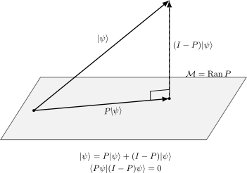
The projector $P$ keeps the component in $\mathcal M$ and $I-P$ keeps the orthogonal component. Their squared norms add to $\|\psi\|^2$.

Three membership tests

The action of $P$ detects whether a vector is in the selected subspace:

$$\begin{aligned} |\psi\rangle\in\operatorname{Ran}P &\iff P|\psi\rangle=|\psi\rangle,\\ |\psi\rangle\in\operatorname{Ker}P &\iff P|\psi\rangle=0,\\ |\psi\rangle\in(\operatorname{Ran}P)^\perp &\iff P|\psi\rangle=0. \end{aligned}$$

Conversely, every closed subspace $\mathcal M$ of a Hilbert space determines a unique orthogonal projector $P_{\mathcal M}$. Closedness matters in infinite dimensions: the nearest point in an arbitrary nonclosed subspace need not belong to that subspace.

Immediate Algebraic Consequences

The defining equations force several useful properties.

Eigenvalues are zero or one

If $P|p\rangle=p|p\rangle$, then

$$p^2|p\rangle = P^2|p\rangle = P|p\rangle = p|p\rangle.$$

Therefore

$$p(p-1)=0,$$

so the only possible eigenvalues are $0$ and $1$. The $1$ eigenspace is $\operatorname{Ran}P$, and the $0$ eigenspace is $\operatorname{Ker}P$.

A projector is positive

For every $|\psi\rangle$,

$$\begin{aligned} \langle\psi|P|\psi\rangle &= \langle\psi|P^2|\psi\rangle\\ &= \langle P\psi|P\psi\rangle\\ &= \|P\psi\|^2 \geq 0. \end{aligned}$$

The complementary projector $I-P$ is also positive, so

$$0\leq P\leq I$$

in the operator order. For a normalized state,

$$0 \leq \langle\psi|P|\psi\rangle \leq 1.$$

This interval is exactly what is needed for a probability.

The complement is another projector

Define

$$P^\perp=I-P.$$

Then

$$(P^\perp)^2=P^\perp, \qquad (P^\perp)^\dagger=P^\perp,$$

and

$$PP^\perp=P^\perp P=0.$$

The range of $P^\perp$ is $(\operatorname{Ran}P)^\perp$.

Norm, rank, and trace

Every orthogonal projector is bounded and defined on the whole Hilbert space. Unless $P=0$, its operator norm is

$$\|P\|_{\mathrm{op}}=1.$$

In finite dimensions,

$$\operatorname{Tr}P = \operatorname{rank}P = \dim(\operatorname{Ran}P),$$

because the eigenvalues consist of one $1$ for each retained dimension and zeros otherwise.

Projection onto a State

For a normalized vector $|\phi\rangle$, the rank-one projector onto its span is

$$P_\phi = |\phi\rangle\langle\phi|.$$

Acting on an arbitrary state gives

$$P_\phi|\psi\rangle = |\phi\rangle \langle\phi|\psi\rangle.$$

The overlap $\langle\phi|\psi\rangle$ is the coefficient of the retained component. Idempotence follows from normalization:

$$\begin{aligned} P_\phi^2 &= |\phi\rangle\langle\phi|\phi\rangle\langle\phi|\\ &= |\phi\rangle\langle\phi|\\ &=P_\phi. \end{aligned}$$

If $|v\rangle\neq0$ is not normalized, the corresponding projector is

$$P_v = \frac{|v\rangle\langle v|}{\langle v|v\rangle}.$$

Omitting the denominator produces an idempotent operator only when $\langle v|v\rangle=1$.

Rays, not phase choices

Replacing $|\phi\rangle$ by $e^{i\alpha}|\phi\rangle$ leaves the projector unchanged:

$$e^{i\alpha}|\phi\rangle \langle\phi|e^{-i\alpha} = |\phi\rangle\langle\phi|.$$

A rank-one projector therefore represents the ray directly. This is one reason density-operator notation is natural even for pure states; see Pure States.

Projection onto a Subspace

Let $\mathcal M$ have an orthonormal basis $\{|e_\alpha\rangle\}$. The orthogonal projector onto $\mathcal M$ is

$$P_{\mathcal M} = \sum_\alpha |e_\alpha\rangle\langle e_\alpha|.$$

For a finite-dimensional subspace this is an ordinary finite sum. For a countably infinite orthonormal basis, the partial sums converge strongly: for each fixed $|\psi\rangle$, the projected vectors converge in norm.

Acting on $|\psi\rangle$ gives

$$P_{\mathcal M}|\psi\rangle = \sum_\alpha |e_\alpha\rangle \langle e_\alpha|\psi\rangle.$$

The result is the unique vector in $\mathcal M$ nearest to $|\psi\rangle$.

Basis independence

The orthonormal basis inside $\mathcal M$ is not unique, but the projector is. If

$$|f_\mu\rangle = \sum_\alpha U_{\mu\alpha}|e_\alpha\rangle$$

with $U$ unitary on the subspace, then

$$\begin{aligned} \sum_\mu|f_\mu\rangle\langle f_\mu| &= \sum_{\alpha,\beta} \left( \sum_\mu U_{\mu\alpha}U_{\mu\beta}^* \right) |e_\alpha\rangle\langle e_\beta|\\ &= \sum_\alpha|e_\alpha\rangle\langle e_\alpha|. \end{aligned}$$

This basis independence is essential for degenerate measurement outcomes. The physical outcome selects an eigenspace, not an arbitrary basis chosen inside it.

A nonorthonormal spanning set

Suppose linearly independent vectors $|v_i\rangle$ span a finite-dimensional subspace but are not orthonormal. With Gram matrix

$$G_{ij}=\langle v_i|v_j\rangle,$$

the orthogonal projector is

$$P = \sum_{i,j} |v_i\rangle (G^{-1})_{ij} \langle v_j|.$$

The inverse Gram matrix is required. The naive sum $\sum_i|v_i\rangle\langle v_i|$ is generally not a projector when the spanning vectors are nonorthogonal.

Orthogonal Families and Resolution of Identity

A family $\{P_a\}$ is mutually orthogonal when

$$P_aP_b = \delta_{ab}P_a.$$

For $a\neq b$, this means every vector in $\operatorname{Ran}P_a$ is orthogonal to every vector in $\operatorname{Ran}P_b$. If the family is complete,

$$\sum_aP_a=I.$$

This is a resolution of the identity. Every state then decomposes as

$$|\psi\rangle = \sum_aP_a|\psi\rangle,$$

with orthogonal components, and

$$\|\psi\|^2 = \sum_a\|P_a\psi\|^2.$$

For an infinite family, the sum is understood in the strong sense. It need not converge in operator norm.

Coarse graining

If $S$ is a set of mutually exclusive outcome labels, then

$$P_S=\sum_{a\in S}P_a$$

is the projector onto the direct sum of their subspaces. Combining several fine outcomes into one reported outcome is therefore represented by adding their orthogonal projectors. Adding nonorthogonal projectors does not generally produce a projector.

Projectors as Yes-No Observables

Because $P$ is self-adjoint and has eigenvalues $0$ and $1$, it is itself a sharp observable. Measuring $P$ asks:

Is the system in the subspace $\operatorname{Ran}P$?

The ideal projective measurement has alternatives

$$\left\lbrace P,\ I-P\right\rbrace.$$

For a normalized pure state, the Born probabilities are

$$\begin{aligned} p(\mathrm{yes}) &= \langle\psi|P|\psi\rangle = \|P\psi\|^2,\\ p(\mathrm{no}) &= \langle\psi|(I-P)|\psi\rangle = \|(I-P)\psi\|^2. \end{aligned}$$

Their sum is one by the orthogonal decomposition. For a density operator $\rho$,

$$p(\mathrm{yes}) = \operatorname{Tr}(\rho P).$$

The canonical probability rule is developed in Born Rule, including what the rule assumes and what it does not settle.

Zero-one and plus-minus-one encodings

The same binary alternative can be labeled by $\pm1$ rather than $0,1$. Define

$$Q=2P-I.$$

Then

$$Q^\dagger=Q, \qquad Q^2=I,$$

and conversely

$$P=\frac{I+Q}{2}.$$

This relation appears for spin observables, parity sectors, stabilizers, and other self-adjoint involutions.

Spectral Projectors and Degeneracy

Let $A$ be a finite-dimensional self-adjoint observable. For each distinct eigenvalue $a$, let $P_a$ project onto the full eigenspace $\mathcal E_a$. Then

$$A=\sum_a aP_a, \qquad \sum_aP_a=I.$$

If $a$ is nondegenerate,

$$P_a=|a\rangle\langle a|.$$

If $a$ has degeneracy $g_a$ and $\{|a,\lambda\rangle\}_{\lambda=1}^{g_a}$ is any orthonormal basis of its eigenspace, then

$$P_a = \sum_{\lambda=1}^{g_a} |a,\lambda\rangle \langle a,\lambda|.$$

The basis vectors inside the eigenspace can change, but $P_a$ cannot. The projector is therefore the invariant object associated with the outcome. See Eigenvalues and Eigenstates for the definite-value statement and Spectral Decomposition for reconstruction of $A$. The spectral relabeling that defines $f(A)$ is developed in Functions of Operators.

Continuous-Spectrum Projectors

Continuous spectra do not eliminate projectors. They replace a sum over normalizable eigenvectors by a projection-valued measure. For a self-adjoint observable $A$ and a Borel set $\Delta\subseteq\mathbb R$, the spectral projector

$$E_A(\Delta)$$

selects the part of the state whose $A$ values lie in $\Delta$. It satisfies

$$\begin{aligned} E_A(\varnothing)&=0,\\ E_A(\mathbb R)&=I,\\ E_A(\Delta_1)E_A(\Delta_2) &= E_A(\Delta_1\cap\Delta_2). \end{aligned}$$

For disjoint sets, the projectors add countably in the strong operator sense. The probability of finding $A$ in $\Delta$ is

$$\Pr(A\in\Delta) = \langle\psi|E_A(\Delta)|\psi\rangle.$$

The measure-theoretic owner for strong countable additivity, scalar state measures, coarse graining, and the PVM–POVM–instrument boundary is Projection-Valued Measures.

For the position operator in one dimension and a spatial region $R$,

$$\bigl(E_X(R)\psi\bigr)(x) = \mathbf 1_R(x)\psi(x),$$

where $\mathbf 1_R$ is the indicator function. This is a genuine bounded projector. By contrast, the formal object $|x\rangle\langle x|$ at one exact position is not a rank-one projector onto a normalizable Hilbert-space vector. The spectral distinction is developed in Discrete and Continuous Spectra.

Products, Intersections, and Compatibility

Let $P$ and $Q$ be orthogonal projectors. If they commute, then

$$PQ=QP$$

is itself an orthogonal projector:

$$(PQ)^2=PQ, \qquad (PQ)^\dagger=PQ.$$

Its range is the intersection,

$$\operatorname{Ran}(PQ) = \operatorname{Ran}P \cap \operatorname{Ran}Q.$$

Conversely, if $PQ$ is an orthogonal projector, self-adjointness gives $PQ=(PQ)^\dagger=QP$. Thus the product of two orthogonal projectors is an orthogonal projector exactly when they commute.

For commuting $P$ and $Q$, the projector onto the closed span of the two subspaces is

$$P\vee Q = P+Q-PQ.$$

If the subspaces are orthogonal, $PQ=0$ and this reduces to $P+Q$.

When $P$ and $Q$ do not commute, $PQ$ is generally neither self-adjoint nor idempotent. The order of filtering matters, and no single intersection projector is represented by the simple product. Compatibility of complete measurements is treated in Compatible Observables.

Inclusion of sharp properties

The relation

$$P\leq Q$$

means that $\operatorname{Ran}P\subseteq\operatorname{Ran}Q$. For orthogonal projectors, this is equivalent to

$$PQ=QP=P.$$

Any state satisfying the sharper property $P$ with certainty then also satisfies $Q$ with certainty.

Worked Examples

Qubit projector along an axis

Let $\boldsymbol n$ be a unit vector and $\boldsymbol\sigma=(\sigma_x,\sigma_y,\sigma_z)$. The projector onto the $+1$ eigenspace of $\boldsymbol n\cdot\boldsymbol\sigma$ is

$$P_{\boldsymbol n,+} = \frac12 \left( I+\boldsymbol n\cdot\boldsymbol\sigma \right).$$

Since

$$(\boldsymbol n\cdot\boldsymbol\sigma)^2=I,$$

one finds

$$P_{\boldsymbol n,+}^2=P_{\boldsymbol n,+}.$$

For a qubit state

$$\rho = \frac12 \left( I+\boldsymbol r\cdot\boldsymbol\sigma \right),$$

the yes probability is

$$\operatorname{Tr} \left( \rho P_{\boldsymbol n,+} \right) = \frac{1+\boldsymbol r\cdot\boldsymbol n}{2}.$$

The geometry of $\boldsymbol r$ is developed in Bloch Sphere.

A degenerate three-level outcome

On an orthonormal basis $\{|1\rangle,|2\rangle,|3\rangle\}$, consider

$$A = a \left( |1\rangle\langle1| +|2\rangle\langle2| \right) +b|3\rangle\langle3|,$$

with $a\neq b$. The outcome projectors are

$$\begin{aligned} P_a &= |1\rangle\langle1| +|2\rangle\langle2|,\\ P_b &= |3\rangle\langle3|. \end{aligned}$$

For a normalized state

$$|\psi\rangle = c_1|1\rangle +c_2|2\rangle +c_3|3\rangle,$$

with

$$\sum_{j=1}^3|c_j|^2=1,$$

the probabilities are

$$\Pr(a)=|c_1|^2+|c_2|^2, \qquad \Pr(b)=|c_3|^2.$$

The result does not depend on which orthonormal basis is chosen inside the two-dimensional $a$ eigenspace.

Parity sectors

If $\Pi$ is a self-adjoint parity operator satisfying $\Pi^2=I$, then

$$P_+ = \frac{I+\Pi}{2}, \qquad P_- = \frac{I-\Pi}{2}$$

project onto the even and odd sectors. They obey

$$P_+P_-=0, \qquad P_++P_-=I.$$

This is the general conversion between a self-adjoint involution and its two spectral projectors.

Projection Is Not Yet a State-Update Rule

The vector $P_a|\psi\rangle$ is the component associated with outcome $a$, but it is generally unnormalized:

$$\|P_a\psi\|^2=p(a).$$

For an ideal selective projective measurement with $p(a)>0$, the Lüders update uses

$$|\psi\rangle \longmapsto \frac{P_a|\psi\rangle}{\sqrt{p(a)}}.$$

That formula requires a measurement model in addition to the operator algebra. Its canonical treatment, including density operators and degenerate outcomes, is Degenerate Measurements and Lüders Rule.

Not every measurement outcome is represented by a projector. A general POVM effect $E_i$ satisfies

$$0\leq E_i\leq I, \qquad \sum_iE_i=I,$$

but need not satisfy $E_i^2=E_i$. See POVMs: First Encounter.

Common Mistakes

• Using idempotence alone to infer orthogonality. The condition $P^2=P$ allows oblique projectors; quantum projectors also satisfy $P^\dagger=P$.
• Forgetting normalization in a rank-one formula. The operator $|v\rangle\langle v|$ is a projector only when $|v\rangle$ is normalized.
• Confusing a vector with its projector. The vectors $|\phi\rangle$ and $e^{i\alpha}|\phi\rangle$ differ, while their rank-one projector is identical.
• Replacing a degenerate outcome by one eigenvector. The outcome projector covers the entire eigenspace.
• Adding arbitrary projectors. The sum $P+Q$ is a projector only when the ranges are orthogonal; for commuting projectors with overlap, use $P+Q-PQ$ for their span.
• Assuming $PQ$ is always a projector. It is an orthogonal projector exactly when $P$ and $Q$ commute.
• Forgetting completeness. A list of alternatives describes an exhaustive projective measurement only when its projectors sum to $I$.
• Calling $P|\psi\rangle$ a probability. The probability is the squared norm $\|P\psi\|^2$; the projected vector is an amplitude-bearing component.
• Treating $|x\rangle\langle x|$ as an ordinary rank-one projector. Exact continuous-spectrum kets are generalized vectors; measurable regions are represented by genuine spectral projectors.
• Building state update into projector algebra. Projection identifies an outcome component. A physical update rule is additional measurement-model structure.

Scope and Canonical Boundaries

This page owns the geometric and physical meaning of orthogonal projectors. Nearby canonical pages carry the next layers:

• Mathematical Projectors treats general idempotent maps and projection algebra.
• Spectral Decomposition reconstructs observables and functions of observables from spectral projectors.
• Born Rule for Discrete Spectra gives the probability workflow for discrete outcomes.
• Projective Measurement specifies ideal measurements and their outcome structure.
• Trace Rule and Expectation Values develops probabilities and expectations for mixed states.
• Compatible Observables treats commuting spectral projectors and joint outcomes.

Summary

• An orthogonal projector satisfies $P^2=P$ and $P^\dagger=P$.
• Its range is a closed subspace, and its kernel is the orthogonal complement.
• Every state decomposes uniquely as $|\psi\rangle=P|\psi\rangle+(I-P)|\psi\rangle$.
• A rank-one projector represents a ray; a higher-rank projector represents a subspace independently of the basis chosen inside it.
• The eigenvalues of a projector are $0$ and $1$, and $\langle\psi|P|\psi\rangle=\|P\psi\|^2$ is a probability for normalized states.
• Mutually orthogonal projectors that sum to $I$ represent exhaustive sharp alternatives.
• Degenerate outcomes correspond to eigenspace projectors, not arbitrary rank-one refinements.
• Continuous observables use spectral projectors $E_A(\Delta)$ for measurable sets of outcomes.
• Products of orthogonal projectors are projectors exactly when the projectors commute.
• Projector algebra identifies outcome components; normalized state update and generalized measurements require additional formalism.

References

• P. Busch, P. J. Lahti, J.-P. Pellonpää, and K. Ylinen, Quantum Measurement, Springer, 2016.
• P. A. M. Dirac, The Principles of Quantum Mechanics, 4th ed., Oxford University Press, 1958.
• B. C. Hall, Quantum Theory for Mathematicians, Springer, 2013.
• M. A. Nielsen and I. L. Chuang, Quantum Computation and Quantum Information, Cambridge University Press, 2010.
• J. J. Sakurai and J. Napolitano, Modern Quantum Mechanics, 3rd ed., Cambridge University Press, 2020.
• R. Shankar, Principles of Quantum Mechanics, 2nd ed., Springer, 1994.
• J. von Neumann, Mathematical Foundations of Quantum Mechanics, Princeton University Press, 1955.

Exercises

Exercise 1: Rank-one projector

Let $|\phi\rangle$ be normalized. Prove that $P_\phi=|\phi\rangle\langle\phi|$ is self-adjoint and idempotent. Determine its range and kernel.

Solution

Taking the adjoint gives

$$P_\phi^\dagger = \left(|\phi\rangle\langle\phi|\right)^\dagger = |\phi\rangle\langle\phi| =P_\phi.$$

Normalization gives

$$P_\phi^2 = |\phi\rangle \langle\phi|\phi\rangle \langle\phi| =P_\phi.$$

Every output is proportional to $|\phi\rangle$, and $P_\phi|\phi\rangle=|\phi\rangle$, so

$$\operatorname{Ran}P_\phi = \operatorname{span}\left\lbrace|\phi\rangle\right\rbrace.$$

The kernel consists of vectors satisfying $\langle\phi|\psi\rangle=0$, hence it is the orthogonal complement of that span.

Exercise 2: An unnormalized vector

Let $|v\rangle\neq0$. Show that

$$P_v = \frac{|v\rangle\langle v|}{\langle v|v\rangle}$$

is a projector. What goes wrong if the denominator is omitted?

Solution

The operator is self-adjoint because the denominator is real and positive. Moreover,

$$\begin{aligned} P_v^2 &= \frac{|v\rangle\langle v|v\rangle\langle v|} {\langle v|v\rangle^2}\\ &= \frac{|v\rangle\langle v|}{\langle v|v\rangle}\\ &=P_v. \end{aligned}$$

Without the denominator,

$$\left(|v\rangle\langle v|\right)^2 = \langle v|v\rangle |v\rangle\langle v|,$$

which equals the original operator only when $|v\rangle$ is normalized.

Exercise 3: Pythagorean decomposition

For an orthogonal projector $P$, prove

$$\|\psi\|^2 = \|P\psi\|^2 + \|(I-P)\psi\|^2.$$

Solution

Write

$$|\psi\rangle = P|\psi\rangle + (I-P)|\psi\rangle.$$

The cross term vanishes:

$$\langle P\psi|(I-P)\psi\rangle = \langle\psi|P(I-P)|\psi\rangle =0.$$

Expanding the squared norm therefore leaves the sum of the two squared norms.

Exercise 4: A qubit projector

Let

$$|+\rangle = \frac{|0\rangle+|1\rangle}{\sqrt2}.$$

Write $P_+=|+\rangle\langle+|$ as a matrix in the computational basis. For

$$|\psi\rangle = \frac{|0\rangle+i|1\rangle}{\sqrt2},$$

compute the yes probability.

Solution

The projector is

$$P_+ = \frac12 \begin{pmatrix} 1&1\\ 1&1 \end{pmatrix}.$$

The overlap is

$$\langle+|\psi\rangle = \frac{1+i}{2},$$

so

$$p(+) = \left|\frac{1+i}{2}\right|^2 = \frac12.$$

Exercise 5: Coarse graining

Suppose $P_1,P_2,P_3$ are mutually orthogonal projectors satisfying

$$P_1+P_2+P_3=I.$$

Show that $P_{12}=P_1+P_2$ is a projector and that $\{P_{12},P_3\}$ is a complete projective measurement.

Solution

Orthogonality gives $P_1P_2=P_2P_1=0$. Therefore

$$\begin{aligned} P_{12}^2 &= (P_1+P_2)^2\\ &= P_1+P_2\\ &=P_{12}. \end{aligned}$$

The sum is self-adjoint, so $P_{12}$ is an orthogonal projector. Also

$$P_{12}P_3=0, \qquad P_{12}+P_3=I.$$

Thus the first two fine outcomes have been combined into one coarse outcome.

Exercise 6: Product of two projectors

Let $P$ and $Q$ be orthogonal projectors. Prove that $PQ$ is an orthogonal projector if and only if $P$ and $Q$ commute.

Solution

If $PQ=QP$, then

$$(PQ)^2 = PQPQ = P^2Q^2 =PQ,$$

and

$$(PQ)^\dagger = QP =PQ.$$

Hence $PQ$ is an orthogonal projector.

Conversely, if $PQ$ is an orthogonal projector, it is self-adjoint. Therefore

$$PQ = (PQ)^\dagger =QP,$$

so $P$ and $Q$ commute.

Exercise 7: Degeneracy and basis independence

Let $P$ project onto a two-dimensional subspace with orthonormal basis $\{|e_1\rangle,|e_2\rangle\}$. Define

$$\begin{aligned} |f_1\rangle &= \frac{|e_1\rangle+|e_2\rangle}{\sqrt2},\\ |f_2\rangle &= \frac{|e_1\rangle-|e_2\rangle}{\sqrt2}. \end{aligned}$$

Verify that

$$|f_1\rangle\langle f_1| +|f_2\rangle\langle f_2| = |e_1\rangle\langle e_1| +|e_2\rangle\langle e_2|.$$

Solution

Expanding the two outer products, the cross terms cancel while each diagonal term appears twice:

$$\begin{aligned} &|f_1\rangle\langle f_1| +|f_2\rangle\langle f_2|\\ &\quad= \frac12 \left( 2|e_1\rangle\langle e_1| +2|e_2\rangle\langle e_2| \right)\\ &\quad= |e_1\rangle\langle e_1| +|e_2\rangle\langle e_2|. \end{aligned}$$

The sum is the original projector. The subspace is physical; the chosen orthonormal basis inside it is not.

Exercise 8: Position in a region

For a normalized wavefunction $\psi\in L^2(\mathbb R)$ and a measurable region $R$, define

$$(P_R\psi)(x) = \mathbf1_R(x)\psi(x).$$

Show that $P_R$ is an orthogonal projector and interpret $\langle\psi|P_R|\psi\rangle$.

Solution

Because $\mathbf1_R(x)^2=\mathbf1_R(x)$,

$$P_R^2=P_R.$$

Multiplication by the real function $\mathbf1_R$ is self-adjoint, so $P_R^\dagger=P_R$. Its expectation value is

$$\begin{aligned} \langle\psi|P_R|\psi\rangle &= \int_{\mathbb R} \psi^*(x)\mathbf1_R(x)\psi(x)\,dx\\ &= \int_R|\psi(x)|^2\,dx. \end{aligned}$$

This is the probability of finding the particle in $R$.