Projection-Valued Measures

A projection-valued measure (PVM) assigns an orthogonal projector to each measurable set of outcomes. It is the operator-valued version of a classical measure appropriate to a sharp quantum observable. If $E:\Sigma\to\mathcal B(\mathcal H)$ is a PVM and $\psi$ is normalized, then

$$\mu_\psi(\Delta) = \langle\psi,E(\Delta)\psi\rangle$$

is an ordinary probability measure on the outcome space. Disjoint outcome sets map to orthogonal subspaces, and countable unions map to strong sums of their projectors.

PVMs unify discrete eigenspace sums and continuous spectral intervals without pretending that every spectral value has a normalizable eigenvector. They also carry less information than a complete measurement model: a PVM fixes sharp event probabilities, not apparatus dynamics or state update.

Required background. The Unbounded Spectral Theorem introduces the unique PVM of a self-adjoint operator; Projectors supplies their geometry. Familiarity with sigma-algebras and countable additivity is assumed.

Helpful background. The Born Rule supplies the state-event probability pairing; the Continuous Born Rule develops measurable outcome sets before probability densities.

A projection measure on an outcome space

Let $(\Omega,\Sigma)$ be a measurable space and $\mathcal H$ a complex Hilbert space. A PVM is a map

$$E:\Sigma\longrightarrow\mathcal B(\mathcal H)$$

such that:

1. $E(\Delta)$ is an orthogonal projection for every $\Delta\in\Sigma$;

2. $E(\varnothing)=0$ and $E(\Omega)=I$;

3. if $\Delta_1,\Delta_2,\ldots$ are pairwise disjoint, then

   $$E\!\left(\bigcup_{n=1}^{\infty}\Delta_n\right)\psi = \sum_{n=1}^{\infty}E(\Delta_n)\psi$$

   for every $\psi\in\mathcal H$, with the series converging in norm.

The last condition is countable additivity in the strong operator topology. It means convergence after acting on each fixed vector. It does not require convergence in operator norm.

Some definitions also state multiplicativity as an axiom. It follows from the projection and additivity conditions:

$$E(\Delta)E(\Gamma) = E(\Delta\cap\Gamma).$$

In particular, disjoint sets have orthogonal projectors,

$$\Delta\cap\Gamma=\varnothing \quad\Longrightarrow\quad E(\Delta)E(\Gamma)=0.$$

Thus classical set logic becomes projection logic within the commuting range of one PVM.

Set operations become projector operations

The axioms imply a useful dictionary:

Outcome-set relation	Projection relation
complement $\Delta^{\mathrm c}$	$E(\Delta^{\mathrm c})=I-E(\Delta)$
intersection $\Delta\cap\Gamma$	$E(\Delta)E(\Gamma)$
disjoint union $\Delta\sqcup\Gamma$	$E(\Delta)+E(\Gamma)$
inclusion $\Delta\subseteq\Gamma$	$E(\Delta)\leq E(\Gamma)$
difference $\Gamma\setminus\Delta$, for $\Delta\subseteq\Gamma$	$E(\Gamma)-E(\Delta)$

The order $P\leq Q$ means $\operatorname{Ran}P\subseteq\operatorname{Ran}Q$, equivalently $PQ=P$. Monotonicity follows by decomposing $\Gamma=\Delta\sqcup(\Gamma\setminus\Delta)$.

For a decreasing sequence $\Delta_n\downarrow\Delta$, continuity of the associated scalar measures gives

$$E(\Delta_n)\psi\longrightarrow E(\Delta)\psi.$$

Similarly, increasing sets converge strongly to the projector of their union. These continuity properties are part of what makes limiting spectral windows well behaved.

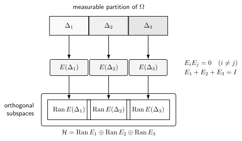
A finite measurable partition illustrates the PVM dictionary: disjoint outcome sets map to mutually orthogonal projectors, and an exhaustive partition resolves the identity. Countable partitions obey the same statement with strong-operator convergence.

Why the sum is strong, not norm convergent

Let $\{e_n\}_{n=0}^{\infty}$ be the standard orthonormal basis of $\ell^2(\mathbb N_0)$. On the measurable space $\mathbb N_0$, define

$$E(S)c = \sum_{n\in S}\langle e_n,c\rangle e_n.$$

For $S_N=\{0,1,\ldots,N\}$,

$$E(S_N)c \longrightarrow c$$

for every $c\in\ell^2$, because the tail of a square-summable sequence tends to zero. Hence $E(S_N)\to I$ strongly.

But

$$\|I-E(S_N)\|=1$$

for every $N$: choose any unit vector $e_m$ with $m>N$. The convergence is never in operator norm. Requiring norm-countable additivity would therefore exclude the elementary spectral decomposition of an infinite discrete spectrum.

States turn a PVM into scalar measures

For $\phi,\psi\in\mathcal H$, define the complex measure

$$\mu_{\phi,\psi}(\Delta) = \langle\phi,E(\Delta)\psi\rangle.$$

In particular,

$$\mu_\psi(\Delta) = \mu_{\psi,\psi}(\Delta) = \langle\psi,E(\Delta)\psi\rangle$$

is positive and satisfies

$$\mu_\psi(\Omega)=\|\psi\|^2.$$

For a normalized state, $\mu_\psi$ is a probability measure. For a density operator $\rho$, the corresponding measure is

$$\mu_\rho(\Delta) = \operatorname{Tr}[\rho E(\Delta)].$$

Countable additivity of the PVM gives countable additivity of every scalar measure. Conversely, the matrix-element measures determine the PVM: if two PVMs have the same $\mu_{\phi,\psi}$ for all pairs, their projections agree.

The probability measure depends on the state; the PVM does not. The PVM encodes one sharp observable, while $\psi$ or $\rho$ encodes the preparation. Confusing these roles obscures the Born pairing.

Discrete and continuous examples

A discrete observable

Suppose mutually orthogonal projections $P_n$ satisfy

$$\sum_nP_n=I$$

strongly. On $\Omega=\{a_n\}$, define

$$E(\Delta) = \sum_{a_n\in\Delta}P_n.$$

This is a PVM. If $A=\sum_n a_nP_n$ on its natural domain, then $E$ is the spectral PVM of $A$. Degeneracy is carried by the rank of $P_n$; a spectral value need not correspond to a one-dimensional subspace.

Position on the real line

On $L^2(\mathbb R)$, define

$$(E_Q(\Delta)\psi)(x) = \mathbf 1_\Delta(x)\psi(x).$$

Indicator multiplication is an orthogonal projection, intersections multiply correctly, and disjoint unions add strongly. The associated state measure is

$$\mu_\psi^Q(\Delta) = \int_\Delta|\psi(x)|^2\,dx.$$

No point projector is needed: for Lebesgue measure, $E_Q(\{x_0\})=0$. Probabilities attach first to measurable regions. A density $|\psi(x)|^2$ is a representation of that measure relative to $dx$, not a probability assigned to one exact point.

Spectral integrals and observables

Given a real measurable function $a:\Omega\to\mathbb R$, the PVM defines

$$A = \int_\Omega a(\omega)\,dE(\omega)$$

on

$$D(A) = \left\{ \psi: \int_\Omega|a(\omega)|^2\,d\mu_\psi(\omega)<\infty \right\}.$$

This operator is self-adjoint. Conversely, the spectral theorem says that every self-adjoint operator arises this way from a unique PVM on $\mathbb R$ with $a(\lambda)=\lambda$.

For a simple function $a=\sum_j a_j\mathbf 1_{\Delta_j}$, the integral is the familiar sum

$$A=\sum_j a_jE(\Delta_j).$$

The general integral is its measure-theoretic completion. The operator domain is not optional when $a$ is unbounded.

Coarse graining and functions of an observable

Let $f:\Omega\to Y$ be measurable, where $Y$ is another measurable outcome space. Relabeling or coarse graining pushes the PVM forward:

$$E^f(B) = E(f^{-1}(B)), \qquad B\subseteq Y\text{ measurable}.$$

For arbitrary $Y$, this construction is a relabeled PVM; it need not define an operator-valued function of $A$. If $E=E_A$ is the spectral PVM of a self-adjoint $A$ and $f:\mathbb R\to\mathbb R$ is Borel measurable, then $E_A^f$ is the spectral PVM of the self-adjoint operator $f(A)$, with the usual natural-domain qualification when $f$ is unbounded. A complex-valued Borel $f$ similarly gives the spectral PVM of the normal operator $f(A)$ on $\mathbb C$. Binning a continuous readout into intervals instead maps each interval to a detector label and should be understood first as coarse graining; assigning numerical values to those labels is an additional choice.

Coarse graining preserves projection-valuedness because preimages preserve unions, complements, and intersections. By contrast, classical randomization or noisy post-processing can produce effects that are not projectors.

PVMs, POVMs, and instruments

A POVM $F$ assigns a positive operator $F(\Delta)$ to each event, with $F(\Omega)=I$ and weak or strong countable additivity. Its effects need not be idempotent:

$$F(\Delta)^2\ne F(\Delta)$$

in general. A PVM is therefore a special, sharp POVM.

Naimark’s dilation theorem represents a POVM as the compression of a PVM on a larger Hilbert space. It does not make the original effects into projections on the original system Hilbert space. The dilation includes an ancilla or extension and is not an equality of the two measurements at the same level of description.

Neither a PVM nor a POVM specifies conditional state change. A measurement instrument assigns completely positive maps to outcome events and contains both probabilities and post-measurement states. The ideal Lüders update is one possible instrument compatible with a PVM, not an axiom of the PVM itself.

Common pitfalls

Demanding operator-norm additivity. Infinite spectral decompositions are normally only strongly additive. The coordinate PVM on $\ell^2$ is the basic counterexample.

Assigning probabilities to exact continuous values. The primitive object is $\mu_\psi(\Delta)$ for measurable sets. A singleton can have probability zero even when its point lies in the spectrum.

Treating a PVM as state dependent. The observable fixes $E$; the state selects one scalar probability measure through the Born pairing.

Equating PVMs and POVMs after dilation. A dilation moves to a larger Hilbert space. It does not turn an unsharp effect into a system projection.

Reading state update from the event projector. The PVM fixes sharp event statistics. An instrument is extra dynamical structure.

Exercises

1. Complement and monotonicity

Derive $E(\Delta^{\mathrm c})=I-E(\Delta)$ and prove that $\Delta\subseteq\Gamma$ implies $E(\Delta)\leq E(\Gamma)$.

Solution

Because $\Delta$ and $\Delta^{\mathrm c}$ are disjoint and cover $\Omega$,

$$I=E(\Omega)=E(\Delta)+E(\Delta^{\mathrm c}).$$

For $\Delta\subseteq\Gamma$, decompose $\Gamma=\Delta\sqcup(\Gamma\setminus\Delta)$. Then

$$E(\Gamma)-E(\Delta) = E(\Gamma\setminus\Delta) \geq0,$$

so $E(\Delta)\leq E(\Gamma)$.

2. Strong but not norm convergence

Complete the proof that the partial coordinate projections $E(S_N)$ converge strongly to $I$ on $\ell^2$ but satisfy $\|I-E(S_N)\|=1$.

Solution

For $c\in\ell^2$,

$$\|[I-E(S_N)]c\|^2 = \sum_{n>N}|c_n|^2 \longrightarrow0.$$

Thus convergence is strong. The difference is an orthogonal projection, so its norm is at most $1$; because it fixes every $e_m$ with $m>N$, its norm is at least $1$.

3. A state probability measure

Show directly that $\mu_\psi(\Delta)=\langle\psi,E(\Delta)\psi\rangle$ is countably additive for a normalized $\psi$.

Solution

For disjoint $\Delta_n$, strong additivity gives

$$E\!\left(\bigcup_n\Delta_n\right)\psi = \sum_nE(\Delta_n)\psi.$$

Taking the continuous inner product with $\psi$ gives

$$\mu_\psi\!\left(\bigcup_n\Delta_n\right) = \sum_n\mu_\psi(\Delta_n).$$

Positivity follows because each $E(\Delta)$ is positive, and normalization follows from $E(\Omega)=I$.

4. Coarse graining a discrete PVM

Let $E$ have outcomes $a_1,a_2,a_3$ with projectors $P_1,P_2,P_3$. Merge $a_1$ and $a_2$ into one label. Find the new PVM and verify that its event operator is a projector.

Solution

The merged event has projector

$$P_{12}=P_1+P_2.$$

Orthogonality gives

$$P_{12}^2 = P_1^2+P_2^2+P_1P_2+P_2P_1 = P_1+P_2=P_{12}.$$

The remaining event has projector $P_3$, and $P_{12}+P_3=I$.

5. The position PVM

For $E_Q(\Delta)=M_{\mathbf 1_\Delta}$ on $L^2(\mathbb R)$, verify $E_Q(\Delta)E_Q(\Gamma)=E_Q(\Delta\cap\Gamma)$ and compute the probability of the bin $[a,b]$.

Solution

Indicator functions multiply according to $\mathbf 1_\Delta\mathbf 1_\Gamma=\mathbf 1_{\Delta\cap\Gamma}$, so the projector identity follows. For normalized $\psi$,

$$\Pr(Q\in[a,b]) = \langle\psi,E_Q([a,b])\psi\rangle = \int_a^b|\psi(x)|^2\,dx.$$

References

• P. Busch, P. Lahti, J.-P. Pellonpää, and K. Ylinen, Quantum Measurement, Springer, 2016.
• M. Reed and B. Simon, Methods of Modern Mathematical Physics, Volume I: Functional Analysis, revised and enlarged ed., Academic Press, 1980.
• G. Teschl, Mathematical Methods in Quantum Mechanics: With Applications to Schrödinger Operators, 2nd ed., American Mathematical Society, 2014.