Effective Hamiltonians and Scale Separation

An effective Hamiltonian is a reduced generator designed to reproduce specified predictions of a more detailed quantum model within a stated regime and accuracy. It may act on a low-energy subspace, on slow degrees of freedom, in a rotating frame, or only at stroboscopic times. Its value is not that it is smaller. Its value is that the discarded physics has been encoded systematically in corrected energies, induced couplings, dressed observables, or controlled error terms.

The word “effective” is incomplete unless four questions have answers:

1. What is retained? A subspace, band, manifold, slow coordinate, or set of resonant states.
2. What is reproduced? Energies, transition amplitudes, scattering poles, slow dynamics, or one-period evolution.
3. In which regime? Below an energy cutoff, away from resonances, for weak coupling, at high drive frequency, or over a specified time window.
4. To what accuracy? An order in a dimensionless ratio, a norm estimate, a leakage probability, or a benchmark against the full model.

This chapter organizes the main constructions. Projection Methods owns exact P/Q block reduction and state reconstruction, Feshbach Projection Formalism owns the continuum and resonance extension of energy-dependent elimination, Schrieffer–Wolff Transformation owns perturbative unitary block diagonalization, Rotating-Wave Approximation owns near-resonant time averaging, and Magnus Expansion together with Floquet-Magnus Expansion owns exponential and periodic effective generators.

Folded Effective Hamiltonians owns the Q-box derivative and folded-diagram route from an energy-dependent model-space equation to one energy-independent interaction.

Adiabatic Elimination owns the dynamical slow–fast reduction, memory and derivative corrections, the detuned Λ system, and trace-preserving effective operators for decaying fast sectors.

Born–Oppenheimer Approximation as Scale Separation owns the heavy–light mass expansion, exact electronic-channel equations, potential-energy surfaces, and diagnostics for nonadiabatic failure.

Average Hamiltonian Theory owns periodic control cycles, toggling-frame interval averages, pulse-order corrections, and selective interaction engineering.

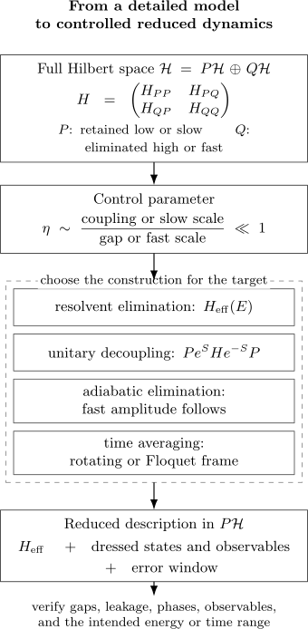
Scale separation can be spectral, dynamical, or temporal. Projection with a resolvent, unitary block diagonalization, adiabatic elimination, and time averaging answer different questions, but each must carry the retained sector, expansion parameter, transformed observables, and error window into the reduced model.

What an Effective Hamiltonian Promises

Let $\mathcal H_{\mathrm{full}}$ be the Hilbert space of the detailed model and $\mathcal H_P$ the retained model space. An encoding isometry

$$\mathcal E: \mathcal H_P \longrightarrow \mathcal H_{\mathrm{full}}$$

identifies reduced states with physical states. A useful effective Hamiltonian satisfies a relation of the form

$$\mathcal E^\dagger e^{-iHt/\hbar} \mathcal E \simeq e^{-iH_{\mathrm{eff}}t/\hbar}$$

for the states, observables, and times of interest. The symbol $\simeq$ hides the entire approximation problem. It may mean equality of selected eigenvalues through order $\eta^k$, agreement of matrix elements up to an error $\varepsilon$, or equality only at integer multiples of a drive period.

No single reduced operator is required to reproduce every property of the full theory. Common targets include:

• the low-lying spectrum and level splittings;
• transition amplitudes among a selected group of states;
• projected Green functions and resonance poles;
• slow evolution after fast transients have decayed;
• dynamics in a rotating frame near a chosen resonance;
• one-period or stroboscopic evolution in a driven system.

The target determines the construction. A Hamiltonian optimized for low-energy eigenvalues need not reproduce short-time leakage. A stroboscopic Floquet Hamiltonian does not by itself describe micromotion inside each period. An energy-dependent optical Hamiltonian can reproduce a projected scattering resolvent without being a conventional Hermitian operator with a fixed spectrum.

Reduction is not deletion

Simply replacing $H$ by its upper-left block can miss the leading physics. States outside the retained space may be only virtually occupied, yet excursions through them can shift energies and mediate interactions. Effective theory keeps those consequences while avoiding explicit evolution of the remote states.

For this reason,

$$H_{\mathrm{eff}} \ne PHP$$

in general. The projected Hamiltonian $PHP$ is only the zeroth approximation. Corrections record how the eliminated sector reacts to the retained one.

Subspaces and Energy Scales

Choose orthogonal projectors

$$\begin{aligned} P^2=P, &\qquad Q^2=Q, \\ P+Q=I, &\qquad PQ=0. \end{aligned}$$

In the decomposition

$$\mathcal H = P\mathcal H \oplus Q\mathcal H,$$

the Hamiltonian has block form

$$H = \begin{pmatrix} H_{PP} & H_{PQ}\\ H_{QP} & H_{QQ} \end{pmatrix},$$

with $H_{PP}=PHP$ and similarly for the other blocks.

Suppose the retained states occupy an energy window separated from the unwanted states by a gap or detuning $\Delta$, while the off-diagonal coupling has characteristic size $v$. The natural expansion parameter is

$$\eta = \frac{v}{\Delta}.$$

When $\eta\ll1$, leakage amplitudes are often of order $\eta$, leakage probabilities of order $\eta^2$, and virtual energy shifts of order

$$\delta E \sim \frac{v^2}{\Delta}.$$

These scalings explain why “unoccupied” levels can matter. Their real population is small, but the phase accumulated from virtual excursions can be measurable over long times.

Choosing the model space

The retained space should contain every state that mixes strongly on the scale being resolved. If two levels have detuning $\delta$ comparable with their coupling $v$, placing one in $P$ and one in $Q$ creates a denominator of order $\delta$ and destroys the expansion. Both belong in the model space and should be diagonalized together.

This is the central rule of Quasi-Degenerate Perturbation Theory:

Model-space rule: treat nearby states exactly; eliminate remote states perturbatively.

The boundary of $P$ is therefore physical and resolution dependent. A two-level model can be excellent for microwave dynamics and inadequate for a faster pulse that resolves leakage levels.

Projection and Resolvent Elimination

For an exact eigenstate,

$$H\lvert\Psi\rangle = E\lvert\Psi\rangle,$$

write

$$\lvert\psi_P\rangle = P\lvert\Psi\rangle, \qquad \lvert\psi_Q\rangle = Q\lvert\Psi\rangle.$$

Projection gives

$$\begin{aligned} H_{PP}\lvert\psi_P\rangle + H_{PQ}\lvert\psi_Q\rangle &= E\lvert\psi_P\rangle, \\ H_{QP}\lvert\psi_P\rangle + H_{QQ}\lvert\psi_Q\rangle &= E\lvert\psi_Q\rangle. \end{aligned}$$

Whenever the required inverse exists with the appropriate boundary condition,

$$\lvert\psi_Q\rangle = \left( E-H_{QQ} \right)^{-1} H_{QP}\lvert\psi_P\rangle.$$

Substitution yields the exact projected equation

$$H_{\mathrm{eff}}(E) \lvert\psi_P\rangle = E\lvert\psi_P\rangle,$$

with

$$\begin{aligned} H_{\mathrm{eff}}(E) &= H_{PP} \\ &\quad+ H_{PQ} \left( E-H_{QQ} \right)^{-1} H_{QP}. \end{aligned}$$

The second term is a self-energy. It contains virtual propagation through $Q$. This formula is exact but nonlinear in $E$, and singularities of the $Q$-space resolvent can invalidate a naive expansion.

For a continuum with outgoing boundary conditions, the resolvent can acquire an imaginary part. The projected operator then becomes non-Hermitian and describes shifts together with resonance widths. That is a feature of the boundary-value problem, not a loss of unitarity in the full closed theory.

The exact block reduction, Schur-complement identity, state reconstruction, and projected normalization are developed in Projection Methods. Continuum boundary conditions, resonance interpretation, and scattering applications belong to Feshbach Projection Formalism.

Perturbative Block Diagonalization

An alternative is to seek a unitary transformation that decouples $P$ and $Q$ to a chosen order. Let $S^\dagger=-S$ and define

$$\widetilde H = e^SHe^{-S}.$$

The generator is chosen so that

$$P\widetilde H Q = O(\eta^{k+1})$$

after working through order $\eta^k$. The effective Hamiltonian is then

$$H_{\mathrm{eff}} = P\widetilde H P.$$

Expanding the exponential produces nested commutators:

$$\widetilde H = H + [S,H] + \frac12[S,[S,H]] + \cdots.$$

Unlike the exact resolvent form, a Schrieffer–Wolff Hamiltonian can be made energy independent and Hermitian order by order for an isolated Hermitian problem. It is especially useful when one wants a reusable low-energy operator rather than a nonlinear eigenvalue equation.

Different block-diagonalization conventions can produce different-looking Hamiltonians related by a unitary transformation inside $P$. Their matrix entries are not individually observable. Spectra and consistently transformed matrix elements are.

Eliminating Fast Degrees of Freedom

Scale separation can be dynamical rather than purely spectral. Consider slow amplitudes $c_s$ coupled to a fast, far-detuned amplitude $c_f$:

$$\begin{aligned} i\dot c_s &= h_{ss}c_s + v_{sf}c_f, \\ i\dot c_f &= \Delta c_f + v_{fs}c_s. \end{aligned}$$

If $\lvert\Delta\rvert$ is the dominant frequency and $c_s$ changes little during a time $\lvert\Delta\rvert^{-1}$, the fast amplitude follows approximately:

$$c_f \simeq - \frac{v_{fs}}{\Delta} c_s.$$

Substitution gives

$$i\dot c_s \simeq \left( h_{ss} - \frac{v_{sf}v_{fs}}{\Delta} \right)c_s.$$

This is adiabatic elimination. The correction is the same virtual second-order process seen in projector and unitary languages. What differs is the organizing assumption: a fast amplitude is slaved to slow motion.

Setting $\dot c_f=0$ is only the first term of an expansion. Adiabatic Elimination derives the exact transient and memory kernel, local derivative corrections, validity conditions, and the open-system effective jumps. Near resonance, $\Delta$ is no longer fast and the eliminated state must be restored.

The Born–Oppenheimer approximation is a richer version of slow–fast separation. Electronic states are solved at fixed nuclear coordinates, generating potential-energy surfaces, while derivative couplings quantify the failure of perfect separation. A level crossing or small electronic gap can make those nonadiabatic couplings large.

Detuned Three-Level Preview

Two long-lived states can couple through a far-detuned excited state even when that excited state remains weakly populated. Eliminating the excited amplitude generates diagonal ac Stark shifts and an off-diagonal Raman coupling with the scale

$$\Omega_{\mathrm R} \sim \frac{\Omega_1^*\Omega_2}{\Delta}.$$

The induced coupling and light shifts arise at the same perturbative order, while the excited-state population is suppressed by a factor of order $\lvert\Omega/\Delta\rvert^2$. The full convention-sensitive derivation, differential light shift, bright and dark states, and spontaneous-scattering extension belong to Adiabatic Elimination.

The same leading virtual process can be organized as degenerate perturbation theory, a resolvent excursion, Schrieffer–Wolff block diagonalization, or adiabatic elimination. Their distinctions matter in higher-order normalization, observable reconstruction, time dependence, and dissipation.

Time-Dependent Effective Hamiltonians

A time-dependent problem introduces another kind of scale separation: fast oscillations can average away while slow resonant dynamics survives.

Exact frame changes come first

For a unitary frame transformation $R(t)$,

$$H_R(t) = R^\dagger(t)H(t)R(t) - i\hbar R^\dagger(t)\dot R(t).$$

This formula is exact. An approximation begins only when terms in $H_R(t)$ are discarded or averaged. Confusing the frame change with the approximation hides the control parameter.

Near-resonant averaging

In a rotating frame, resonant terms can become slowly varying while counter-rotating terms oscillate near twice the carrier frequency. The rotating-wave approximation drops those fast terms when the coupling and detuning are small compared with the fast frequency and when the observation window does not resolve the omitted micromotion.

The leading neglected effect is often not zero. It can include the Bloch–Siegert shift, leakage, or corrections to the rotation axis. Rotating-Wave Approximation develops those conditions quantitatively.

Average and Floquet generators

For general time dependence, the Magnus Expansion writes evolution as

$$U(t,0) = \exp\left[ \Omega(t) \right],$$

where $\Omega(t)$ is built from time integrals and nested commutators. Over an interval $T$, one may define

$$H_{\mathrm{eff}}^{(T)} = \frac{i\hbar}{T} \Omega(T).$$

For a cyclic pulse sequence, Average Hamiltonian Theory first transforms the internal Hamiltonian into the control toggling frame. Its zeroth-order weighted average selects the retained interaction, while ordered commutators quantify pulse-order and finite-cycle corrections.

For periodic driving, Floquet–Magnus Expansion applies the Magnus series directly to a one-period propagator at a chosen drive phase:

$$U(T,0) = e^{-iH_FT/\hbar}.$$

The Floquet Hamiltonian $H_F$ controls stroboscopic evolution. A separate micromotion operator is needed inside each period. High-Frequency Expansions owns the broader inverse-frequency framework: Floquet-space block diagonalization, the phase-independent van Vleck Hamiltonian, kick-operator dressing, resonant denominators, and local many-body prethermal regimes. Its simplest expansion parameter is schematically

$$\eta_\Omega \sim \frac{J}{\hbar\Omega},$$

where $J$ is a local energy or coupling scale. Resonances and many-body heating can limit the useful time window even when early terms are small.

States and Observables Must Be Dressed

An effective Hamiltonian alone is not a complete reduction. Suppose the transformed state is

$$\lvert\widetilde\Psi\rangle = e^S\lvert\Psi\rangle.$$

If $\lvert\psi_{\mathrm{eff}}\rangle=P\lvert\widetilde\Psi\rangle$, then reconstructing the physical state requires

$$\lvert\Psi\rangle \simeq e^{-S}\lvert\psi_{\mathrm{eff}}\rangle,$$

to the same perturbative order. An observable $O$ must be transformed consistently:

$$O_{\mathrm{eff}} = P e^S O e^{-S}P.$$

Using $H_{\mathrm{eff}}$ with the bare projected observable $POP$ can give the correct energy spectrum and incorrect transition strengths. The missing terms represent the small admixture of eliminated states.

The same warning appears in other languages:

• Feshbach elimination reconstructs $\lvert\psi_Q\rangle$ with the resolvent.
• Adiabatic elimination includes derivative and initial-slip corrections.
• Floquet theory requires micromotion dressing for observables away from stroboscopic times.
• Open-system elimination generally modifies both the Hamiltonian and the effective jump operators.

Validity and Error Discipline

Every reduction should report more than the formal Hamiltonian.

Control parameter

Identify a dimensionless ratio such as

$$\frac{v}{\Delta}, \qquad \frac{\tau_{\mathrm{fast}}}{\tau_{\mathrm{slow}}}, \qquad \frac{J}{\hbar\Omega}.$$

If several gaps or frequencies exist, the smallest relevant denominator controls the worst case.

Leakage

Monitor

$$L(t) = \langle\Psi(t)\rvert Q \lvert\Psi(t)\rangle.$$

Small leakage supports a subspace description, but it is not sufficient by itself. Virtual phase shifts can accumulate while $L(t)$ remains small.

Spectral and dynamical errors

An operator error $\delta H=H_{\mathrm{exact}}-H_{\mathrm{eff}}$ can produce an evolution error that grows with time. Duhamel’s identity gives, for bounded Hermitian generators,

$$\left\| e^{-iH_{\mathrm{exact}}t/\hbar} - e^{-iH_{\mathrm{eff}}t/\hbar} \right\| \le \frac{\lvert t\rvert}{\hbar} \lVert\delta H\rVert.$$

Thus a small energy error does not justify arbitrary evolution times. If $\lVert\delta H\rVert=O(\eta^{k+1})$, the naive useful time can shrink as the desired phase accuracy becomes more demanding.

Resonance checks

Inspect denominators explicitly. A drive, threshold, avoided crossing, or continuum pole can make a nominally remote sector resonant. Near such a point:

• enlarge the retained space;
• change to a resonant frame;
• retain the relevant channel exactly;
• or abandon the expansion in favor of direct numerical evolution.

Independent benchmarks

For a finite model, compare low-energy eigenvalues and eigenvectors with direct diagonalization. For dynamics, compare projected populations, phases, and observables over the intended time window. Vary the cutoff, expansion order, and retained space. A single matching eigenvalue is not enough.

Nonuniqueness and Matching

Effective Hamiltonians are not unique. If $W$ is unitary inside the retained space,

$$\begin{aligned} H_{\mathrm{eff}}' &= W H_{\mathrm{eff}}W^\dagger, \\ O_{\mathrm{eff}}' &= W O_{\mathrm{eff}}W^\dagger, \end{aligned}$$

then all consistently computed predictions agree. Time-dependent frame choices, Floquet gauges, and different perturbative generators create similar representational freedom.

The reliable objects are matched observables, not isolated coefficients. A practical matching procedure is:

1. choose the retained degrees of freedom and operator basis;
2. identify the expansion parameter and symmetries;
3. calculate selected full-model amplitudes or energies;
4. choose effective coefficients so the reduced model reproduces them;
5. estimate the first omitted operators and verify against new observables.

This is the quantum-mechanical precursor of effective field theory. The QFT Bridge: EFT and Effective Hamiltonians explains what changes when infinitely many modes, locality, renormalization, and power counting enter.

Method Roadmap

Physical separation	Natural method	Typical output	Principal warning
Chosen subspace coupled to remote states	Projection or Feshbach method	Energy-dependent self-energy	Resolvent poles and boundary conditions
Several model-space states need one reusable interaction	Folded effective Hamiltonian	Energy-independent model-space operator	Q-box poles, root selection, and induced many-body terms
Low-energy and high-energy blocks with weak mixing	Schrieffer–Wolff transformation	Hermitian energy-independent low-energy Hamiltonian	Transform states and observables
Slow amplitudes coupled to fast amplitudes	Adiabatic elimination	Algebraic slow-sector generator	Initial transients and derivative corrections
Heavy and light coordinates	Born–Oppenheimer method	Potential-energy surfaces	Small gaps and nonadiabatic couplings
Near-resonant and fast counter-rotating terms	Rotating-wave approximation	Slowly varying rotating-frame Hamiltonian	Bloch–Siegert shifts and strong-drive failure
Rapid cyclic pulse control	Average Hamiltonian theory	Toggling-frame cycle Hamiltonian	Commutator corrections and finite pulses
General time-ordered evolution	Magnus expansion	Single exponential generator	Convergence and long-time accumulation
One-period logarithm at a chosen drive phase	Floquet–Magnus expansion	Stroboscopic Hamiltonian	Branch, phase, and micromotion conventions
Off-resonant rapid periodic drive	High-frequency expansions	Effective Hamiltonian plus periodic kick	Resonances, asymptotic truncation, and heating
Weakly occupied decaying sector	Effective open-system operators	Effective Hamiltonian and jump operators	Eliminating only the Hamiltonian is incomplete

These methods can overlap. The same three-level atom can be treated by projection, block diagonalization, or adiabatic elimination. Prefer the formulation whose assumptions and target observable are easiest to state and verify.

Applications Across Quantum Physics

• Elementary quantum mechanics: nearly degenerate levels, double-well doublets, spin–orbit reductions, and low-energy scattering channels.
• Atomic, molecular, and optical physics: Raman transitions, light shifts, dark-state manifolds, rotating frames, cavity-mediated interactions, and Born–Oppenheimer surfaces.
• Quantum information: qubit subspaces, leakage corrections, dispersive gates, and perturbative gadgets, together with pulse averaging.
• Quantum matter: the exact Hubbard-dimer superexchange benchmark and effective masses, many-body lattice and impurity reductions, projected bands, and high-frequency Hamiltonian engineering.
• Nuclear physics: model-space interactions, optical potentials, folded Hamiltonians, and reaction channels.
• Open quantum systems: eliminated excited states can induce both coherent shifts and dissipative jump processes.
• Quantum field theory: integrating out heavy modes produces symmetry-allowed effective operators whose coefficients are fixed by matching.

The common logic is scale aware rather than field specific: retain what the experiment resolves, encode what it does not, and carry an error estimate.

Common Mistakes

• Calling $PHP$ the effective Hamiltonian without checking virtual $Q$-space corrections.
• Eliminating a state whose detuning is comparable with its coupling.
• Quoting a small coupling without dividing by the relevant gap or frequency.
• Matching eigenvalues while leaving states and observables undressed.
• Treating an energy-dependent Feshbach operator as an ordinary fixed Hermitian Hamiltonian.
• Setting a fast derivative to zero without estimating derivative and initial-transient corrections.
• Using a rotating-wave or high-frequency Hamiltonian without specifying the frame or observation times.
• Ignoring micromotion because stroboscopic evolution is accurate.
• Assuming small leakage guarantees small phase error.
• Extrapolating a finite-order Hamiltonian to arbitrarily long times.
• Comparing coefficients from two effective Hamiltonians without checking whether they are related by a unitary change of basis.
• Forgetting that open-system elimination changes dissipative operators as well as coherent dynamics.

Exercises

1. Derive the exact projected equation

Starting from the block eigenvalue equation, eliminate $\lvert\psi_Q\rangle$ and derive $H_{\mathrm{eff}}(E)$.

Solution

The projected equations are

$$\begin{aligned} H_{PP}\lvert\psi_P\rangle + H_{PQ}\lvert\psi_Q\rangle &= E\lvert\psi_P\rangle, \\ H_{QP}\lvert\psi_P\rangle + H_{QQ}\lvert\psi_Q\rangle &= E\lvert\psi_Q\rangle. \end{aligned}$$

Rearranging the second equation gives

$$\left( E-H_{QQ} \right)\lvert\psi_Q\rangle = H_{QP}\lvert\psi_P\rangle.$$

Assuming the required resolvent exists,

$$\lvert\psi_Q\rangle = \left( E-H_{QQ} \right)^{-1} H_{QP}\lvert\psi_P\rangle.$$

Substitution into the first equation yields

$$\begin{aligned} H_{\mathrm{eff}}(E) &\equiv H_{PP} \\ &\quad+ H_{PQ} R_Q(E) H_{QP}, \\ R_Q(E) &\equiv \left( E-H_{QQ} \right)^{-1}, \\ H_{\mathrm{eff}}(E) \lvert\psi_P\rangle &= E\lvert\psi_P\rangle. \end{aligned}$$

The first two rows define the effective Hamiltonian and the $Q$-space resolvent.

2. Eliminate one remote level

Let

$$H = \begin{pmatrix} 0 & v\\ v^* & \Delta \end{pmatrix}, \qquad \lvert v\rvert\ll\lvert\Delta\rvert.$$

Take the first basis state as $P$. Find the exact energy-dependent effective Hamiltonian and the low-energy eigenvalue through second order.

Solution

Here

$$\begin{aligned} H_{PP}=0, &\qquad H_{QQ}=\Delta, \\ H_{PQ}=v, &\qquad H_{QP}=v^*. \end{aligned}$$

Therefore

$$H_{\mathrm{eff}}(E) = \frac{\lvert v\rvert^2}{E-\Delta}.$$

The eigenvalue equation is

$$E = \frac{\lvert v\rvert^2}{E-\Delta},$$

or

$$E^2-\Delta E-\lvert v\rvert^2=0.$$

For the root near zero, expand the denominator using $E/\Delta=O(\lvert v/\Delta\rvert^2)$:

$$E_{\mathrm{low}} = - \frac{\lvert v\rvert^2}{\Delta} + O\left( \frac{\lvert v\rvert^4}{\Delta^3} \right).$$

The sign reverses if the eliminated state lies below rather than above the retained state.

3. Diagnose a Raman reduction

A three-level Λ system has Rabi frequencies $\Omega_1$ and $\Omega_2$, one-photon detuning $\Delta$, two-photon detuning $\delta$, and excited-state linewidth $\Gamma$. State the dimensionless ratios that must be small for a coherent two-state reduction, and identify what must be added if spontaneous emission cannot be neglected.

Solution

At minimum,

$$\frac{\lvert\Omega_1\rvert}{\lvert\Delta\rvert}, \quad \frac{\lvert\Omega_2\rvert}{\lvert\Delta\rvert}, \quad \frac{\lvert\delta\rvert}{\lvert\Delta\rvert} \ll 1.$$

Drive-envelope frequencies must also be small compared with $\lvert\Delta\rvert$, and the intended duration must not amplify neglected phase errors. If $\Gamma$ matters, the fast response uses the complex scale $\Delta-i\Gamma/2$, but a non-Hermitian Hamiltonian alone is incomplete. Effective Lindblad jump operators must be retained to describe scattering and preserve trace. The canonical derivation is in Adiabatic Elimination.

4. Bound the dynamical error

Let $H_1$ and $H_2$ be bounded Hermitian operators. Use Duhamel’s identity to show

$$\left\| e^{-iH_1t/\hbar} - e^{-iH_2t/\hbar} \right\| \le \frac{\lvert t\rvert}{\hbar} \lVert H_1-H_2\rVert.$$

Solution

Define

$$F(s) = e^{-iH_1(t-s)/\hbar} e^{-iH_2s/\hbar}.$$

Then

$$\frac{dF}{ds} = \frac{i}{\hbar} e^{-iH_1(t-s)/\hbar} \left( H_1-H_2 \right) e^{-iH_2s/\hbar}.$$

Integrating from $0$ to $t$ gives the difference of the two propagators. Unitary invariance of the operator norm implies

$$\left\| \frac{dF}{ds} \right\| \le \frac{1}{\hbar} \lVert H_1-H_2\rVert.$$

The triangle inequality for the integral then yields the stated bound. It makes explicit why a small generator error can accumulate over long times.

5. Dress an observable

Let $S=O(\eta)$ be anti-Hermitian. Expand

$$O_{\mathrm{eff}} = P e^S O e^{-S}P$$

through first order. Under what condition is $POP$ sufficient to that order?

Solution

The Baker–Campbell–Hausdorff expansion gives

$$e^S O e^{-S} = O+[S,O]+O(\eta^2).$$

Therefore

$$O_{\mathrm{eff}} = POP + P[S,O]P + O(\eta^2).$$

The bare projection $POP$ is sufficient through first order only if

$$P[S,O]P=0.$$

This can occur because of symmetry or block structure, but it should be checked rather than assumed.

6. Choose the retained space

Three unperturbed levels have energies $0$, $\delta$, and $\Delta$, with couplings of characteristic size $v$. Assume

$$\delta\sim v, \qquad v\ll\Delta.$$

Which levels belong in $P$, and what is the natural perturbative parameter?

Solution

The levels at $0$ and $\delta$ are separated by an amount comparable with their coupling. They mix strongly and must both be retained:

$$P = \lvert0\rangle\langle0\rvert + \lvert\delta\rangle\langle\delta\rvert.$$

The level at $\Delta$ is remote and belongs in $Q$. Coupling to it can be expanded in

$$\eta \sim \frac{v}{\Delta}.$$

Inside $P$, the detuning $\delta$ and coupling $v$ should be diagonalized together. Expanding in $v/\delta$ would be uncontrolled because that ratio is of order unity.

Cross-Links

• Projectors
• Small Parameters and Error Estimates
• Quasi-Degenerate Perturbation Theory
• Projection Methods
• Folded Effective Hamiltonians
• Adiabatic Elimination
• Feshbach Projection Formalism
• Schrieffer–Wolff Transformation
• Rotating-Wave Approximation
• Average Hamiltonian Theory
• Magnus Expansion
• Floquet–Magnus Expansion
• High-Frequency Expansions
• Effective Hamiltonians in Quantum Information
• Effective Hamiltonians in Quantum Matter
• QFT Bridge: EFT and Effective Hamiltonians
• Matrix Diagonalization

References

1. H. Feshbach, “Unified theory of nuclear reactions,” Annals of Physics 5, 357–390 (1958).
2. H. Feshbach, “A unified theory of nuclear reactions. II,” Annals of Physics 19, 287–313 (1962).
3. J. R. Schrieffer and P. A. Wolff, “Relation between the Anderson and Kondo Hamiltonians,” Physical Review 149, 491–492 (1966).
4. S. Bravyi, D. P. DiVincenzo, and D. Loss, “Schrieffer–Wolff transformation for quantum many-body systems,” Annals of Physics 326, 2793–2826 (2011).
5. C. Bloch, “Sur la théorie des perturbations des états liés,” Nuclear Physics 6, 329–347 (1958).
6. C. Cohen-Tannoudji, J. Dupont-Roc, and G. Grynberg, Atom–Photon Interactions: Basic Processes and Applications, Wiley (1992).
7. F. Reiter and A. S. Sørensen, “Effective operator formalism for open quantum systems,” Physical Review A 85, 032111 (2012).
8. S. Blanes, F. Casas, J. A. Oteo, and J. Ros, “The Magnus expansion and some of its applications,” Physics Reports 470, 151–238 (2009).
9. N. Goldman and J. Dalibard, “Periodically driven quantum systems: Effective Hamiltonians and engineered gauge fields,” Physical Review X 4, 031027 (2014); see also the published erratum.
10. A. Eckardt and E. Anisimovas, “High-frequency approximation for periodically driven quantum systems from a Floquet-space perspective,” New Journal of Physics 17, 093039 (2015).
11. S. Teufel, Adiabatic Perturbation Theory in Quantum Dynamics, Springer (2003).
12. P. W. Anderson, “Antiferromagnetism. Theory of superexchange interaction,” Physical Review 79, 350–356 (1950).