Folded Effective Hamiltonians

An exact projection of the Schrödinger equation produces an effective Hamiltonian that depends on the energy being sought. A folded effective Hamiltonian reorganizes that energy dependence into an energy-independent operator acting on a chosen model space. In many-body perturbation theory, the extra terms generated by this reorganization are called folded diagrams.

The method solves a practical problem. A shell-model, multireference, or valence-space calculation should diagonalize one matrix and obtain several target states. It is inconvenient to assign a different nonlinear Hamiltonian to every eigenvalue. Folding converts the feedback of the unknown energy into derivatives and repeated insertions of an energy-dependent vertex, traditionally called the Q-box.

This is a specialized extension of Projection Methods, which owns the exact P/Q reduction and state reconstruction. Brillouin–Wigner Perturbation Theory owns the energy-dependent perturbative eigenvalue equation. Schrieffer–Wolff Transformation constructs an energy-independent Hamiltonian by perturbative block diagonalization instead of Q-box folding.

The Energy-Independent Target

Let $P$ project onto a $d$-dimensional model space and let $Q=I-P$. Select $d$ exact eigenstates,

$$H\lvert\Psi_k\rangle = E_k\lvert\Psi_k\rangle, \qquad k=1,\ldots,d,$$

whose projected vectors

$$\lvert\phi_k\rangle = P\lvert\Psi_k\rangle$$

are linearly independent. They need not be orthogonal. Introduce biorthogonal dual vectors in $P\mathcal H$ satisfying

$$\langle\widetilde\phi_j\vert\phi_k\rangle = \delta_{jk}, \qquad \sum_{k=1}^{d} \lvert\phi_k\rangle \langle\widetilde\phi_k\vert = P.$$

An exact energy-independent model-space Hamiltonian is then

$$H_{\mathrm{eff}} = \sum_{k=1}^{d} E_k \lvert\phi_k\rangle \langle\widetilde\phi_k\vert.$$

It obeys

$$H_{\mathrm{eff}} \lvert\phi_k\rangle = E_k\lvert\phi_k\rangle.$$

This formula defines the target but does not yet make it computable: it uses the exact eigenvalues and projected eigenvectors one was trying to find. Folded-diagram methods construct the same kind of operator from perturbative model-space vertices.

Two lessons are already visible:

• the effective Hamiltonian depends on which $d$ exact states are selected;
• it is generally non-Hermitian because the projected eigenvectors are generally nonorthogonal.

An energy-independent effective Hamiltonian is therefore not unique. Similarity transformations within $P\mathcal H$ can change its matrix elements without changing the selected spectrum.

Degenerate Model-Space Setup

The cleanest folded expansion assumes a degenerate unperturbed model space. Write

$$H = H_0+V,$$

with

$$PH_0P = \epsilon_0P, \qquad PH_0Q = QH_0P = 0.$$

Define the energy-dependent Q-box by

$$\begin{aligned} \widehat{\mathcal Q}(\omega) &= PVP \\ &\quad+ PVQ \left( \omega-QHQ \right)^{-1} QVP. \end{aligned}$$

The calligraphic symbol distinguishes the Q-box $\widehat{\mathcal Q}$ from the complementary projector $Q$. Many papers write the vertex simply as $\widehat Q$.

The exact projected equation is

$$\left[ \epsilon_0P + \widehat{\mathcal Q}(E) \right] \lvert\phi\rangle = E\lvert\phi\rangle.$$

This is the Bloch–Horowitz or Brillouin–Wigner form specialized to the degenerate model space. The first term in the Q-box acts directly inside $P$. The resolvent term leaves $P$, propagates entirely inside $Q$, and returns.

The Q-box has poles at eigenvalues of $QHQ$. It is therefore not an ordinary constant interaction. Its variation with $\omega$ measures how strongly the eliminated sector reacts when the target energy changes.

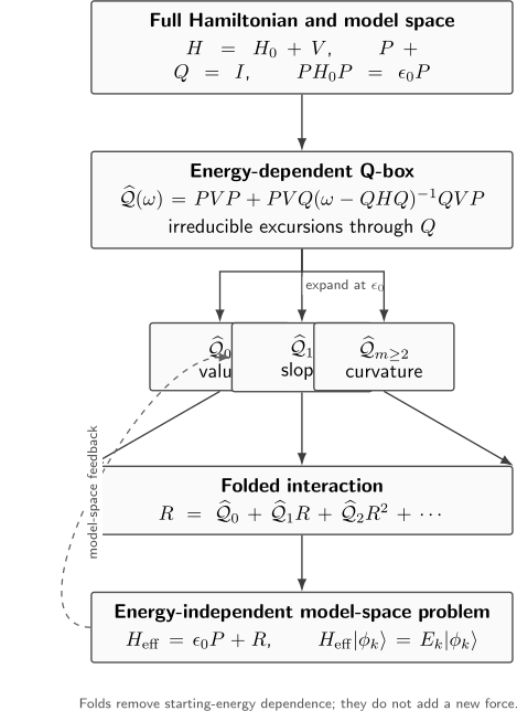
The Q-box contains irreducible excursions through $Q$. Expanding it about $\epsilon_0$ produces derivative vertices $\widehat{\mathcal Q}_m$. Feeding the model-space interaction $R$ back through those vertices sums folded contributions and yields $H_{\mathrm{eff}}=\epsilon_0P+R$.

Trading Energy Dependence for Folds

Write the desired energy-independent Hamiltonian as

$$H_{\mathrm{eff}} = \epsilon_0P+R.$$

For a selected model-space eigenvector,

$$R\lvert\phi_k\rangle = r_k\lvert\phi_k\rangle, \qquad r_k = E_k-\epsilon_0.$$

The energy-dependent equation requires

$$R\lvert\phi_k\rangle = \widehat{\mathcal Q} \left( \epsilon_0+r_k \right) \lvert\phi_k\rangle.$$

Assume the Q-box is analytic between $\epsilon_0$ and the selected energies. Define its normalized derivatives by

$$\widehat{\mathcal Q}_m = \left. \frac{1}{m!} \frac{d^m\widehat{\mathcal Q}} {d\omega^m} \right|_{\omega=\epsilon_0}.$$

For $m\ge1$,

$$\begin{aligned} \widehat{\mathcal Q}_m &= (-1)^m PVQ \\ &\quad\times \left( \epsilon_0-QHQ \right)^{-(m+1)} QVP. \end{aligned}$$

Taylor expansion gives

$$\begin{aligned} \widehat{\mathcal Q} \left( \epsilon_0+r_k \right) \lvert\phi_k\rangle &= \sum_{m=0}^{\infty} \widehat{\mathcal Q}_m r_k^m \lvert\phi_k\rangle \\ &= \sum_{m=0}^{\infty} \widehat{\mathcal Q}_m R^m \lvert\phi_k\rangle. \end{aligned}$$

If the selected vectors span $P\mathcal H$, the operator equation is

$$R = \widehat{\mathcal Q}_0 + \widehat{\mathcal Q}_1R + \widehat{\mathcal Q}_2R^2 + \cdots.$$

This is the algebraic core of folding. The order of the factors matters: $R^m$ acts first on a model-space state, and the derivative vertex acts afterward. The formula is simplest for a degenerate model space; nondegenerate spaces require multi-energy or generalized constructions rather than blind reuse of this equation.

What a fold represents

The Q-box is built to exclude model-space intermediate propagation from its internal resolvent. Yet the exact energy entering the Q-box already contains the model-space interaction $R$. Expanding in that energy feeds model-space propagation back into the vertex. Diagrammatically, joining irreducible vertices across such a model-space propagation folds one contribution over another.

Recursive substitution generates terms of the form

$$\begin{aligned} R &= \widehat{\mathcal Q}_0 + \widehat{\mathcal Q}_1 \widehat{\mathcal Q}_0 \\ &\quad+ \widehat{\mathcal Q}_2 \widehat{\mathcal Q}_0^2 + \widehat{\mathcal Q}_1^2 \widehat{\mathcal Q}_0 + \cdots. \end{aligned}$$

This line displays representative early structures, not a complete truncation rule. A consistent many-body calculation organizes terms by perturbative order, number of folds, or a specified iteration scheme.

Folding does not describe an additional physical interaction. It removes the starting-energy dependence and corrects the counting of model-space intermediate propagation. Omitting folds while retaining a truncated Q-box generally leaves an effective interaction that depends on the arbitrary starting energy $\epsilon_0$.

Iterative Constructions

The simplest fixed-point iteration is

$$\begin{aligned} R^{(0)} &= \widehat{\mathcal Q}_0, \\ R^{(n+1)} &= \widehat{\mathcal Q}_0 + \sum_{m=1}^{\infty} \widehat{\mathcal Q}_m \left[ R^{(n)} \right]^m. \end{aligned}$$

This expression is pedagogically transparent but is not the only practical summation. Kuo–Krenciglowa and Lee–Suzuki constructions reorganize the same derivative information with different iteration maps and root-selection properties.

For the degenerate Lee–Suzuki recursion, the first two interaction iterates can be written

$$\begin{aligned} R_1 &= \widehat{\mathcal Q}_0, \\ R_2 &= \left( I_P-\widehat{\mathcal Q}_1 \right)^{-1} \widehat{\mathcal Q}_0. \end{aligned}$$

The inverse in $R_2$ already sums repeated first-derivative insertions. Higher iterates include higher Q-box derivatives and ordered products of earlier iterates.

Iteration is not merely an implementation detail. In common degenerate formulations, Kuo–Krenciglowa-type iterations are associated with eigenstates having substantial model-space overlap, while the standard Lee–Suzuki construction is organized around eigenvalues near the chosen starting energy. Precise selection and convergence depend on the variant, the projector, and the spectrum. A method name alone does not guarantee that the desired roots will be obtained.

For a scalar fixed-point equation $r=F(r)$, local iteration converges only if

$$\left| F'(r_*) \right| \lt1$$

at the target root. The operator problem has a corresponding stability analysis involving the derivative of the iteration map. Large Q-box derivatives are therefore a direct warning sign.

Worked Example: Folds in a Two-Level Model

Consider

$$H = \begin{pmatrix} \epsilon_0 & g \\ g^* & \epsilon_q \end{pmatrix},$$

and retain the first state. Let

$$D = \epsilon_0-\epsilon_q.$$

The Q-box is the scalar

$$\widehat{\mathcal Q}(\omega) = \frac{\lvert g\rvert^2} {\omega-\epsilon_q}.$$

Writing $E=\epsilon_0+r$, the exact projected equation becomes

$$r = \frac{\lvert g\rvert^2} {D+r}.$$

Expansion about $r=0$ gives

$$\begin{aligned} r &= \frac{\lvert g\rvert^2}{D} - \frac{\lvert g\rvert^2}{D^2}r \\ &\quad+ \frac{\lvert g\rvert^2}{D^3}r^2 - \cdots. \end{aligned}$$

The first Q-box term gives

$$r^{(2)} = \frac{\lvert g\rvert^2}{D}.$$

Feeding it through the first derivative gives the first folded correction,

$$\widehat{\mathcal Q}_1 \widehat{\mathcal Q}_0 = - \frac{\lvert g\rvert^4}{D^3}.$$

At sixth order, two feedback structures contribute:

$$\begin{aligned} \widehat{\mathcal Q}_1^2 \widehat{\mathcal Q}_0 &= \frac{\lvert g\rvert^6}{D^5}, \\ \widehat{\mathcal Q}_2 \widehat{\mathcal Q}_0^2 &= \frac{\lvert g\rvert^6}{D^5}. \end{aligned}$$

Therefore

$$\begin{aligned} r &= \frac{\lvert g\rvert^2}{D} - \frac{\lvert g\rvert^4}{D^3} \\ &\quad+ 2\frac{\lvert g\rvert^6}{D^5} + O\!\left( \frac{\lvert g\rvert^8}{D^7} \right). \end{aligned}$$

The exact root connected continuously to the retained level is

$$r = \frac{ -D + \operatorname{sgn}(D) \sqrt{ D^2+4\lvert g\rvert^2 } }{2}.$$

Its expansion agrees with the folded series for either sign of nonzero $D$. The Q-box has a pole at $r=-D$, so the Taylor series requires

$$\left| \frac{r}{D} \right| \lt1.$$

This example isolates the meaning of a fold: it generates the higher-order consequences of evaluating the self-energy at the shifted energy rather than at the unperturbed one.

Linked and Irreducible Many-Body Vertices

In nuclear shell-model and atomic many-body applications, the Q-box is not evaluated as one exact resolvent. It is expanded in diagrams. The standard construction retains contributions that are:

• valence linked, so every disconnected piece is connected to a valence line;
• irreducible with respect to the model space, so intermediate states internal to the Q-box lie outside $P$;
• evaluated to a stated order in the residual interaction.

Folded diagrams then restore the model-space feedback needed to create an energy-independent interaction while preserving linked structure. The detailed graphical rules depend on the many-body formalism and are not identical to merely multiplying two ordinary Feynman diagrams.

The bookkeeping has a second layer. Even if the starting interaction is two-body, eliminating degrees of freedom generally induces three-body and higher-body operators in the model space. A valence-space Hamiltonian truncated at the two-body level therefore makes a cluster approximation in addition to truncating the Q-box and folded series.

This hierarchy should be reported separately:

1. order used for the irreducible Q-box;
2. method used to sum its folds;
3. maximum particle rank retained in the effective Hamiltonian;
4. numerical model-space and intermediate-state cutoffs.

Agreement after varying only one of these choices does not establish convergence in the others.

Non-Hermiticity and Hermitization

The standard energy-independent Hamiltonian built from projected exact eigenvectors is generally non-Hermitian. This is not caused by an underlying non-Hermitian full Hamiltonian. It arises because projection makes the model-space eigenvectors nonorthogonal and the decoupling transformation need not be unitary.

Let the wave operator be

$$\Omega = P+\chi, \qquad \chi = Q\chi P,$$

so that selected full states satisfy

$$\lvert\Psi_k\rangle = \Omega\lvert\phi_k\rangle.$$

Their model-space norm operator is

$$M = \Omega^\dagger\Omega = I_P+\chi^\dagger\chi.$$

For an exact decoupling construction, the non-Hermitian effective Hamiltonian is quasi-Hermitian:

$$H_{\mathrm{eff}}^\dagger M = M H_{\mathrm{eff}}.$$

A Hermitian representative is then

$$H_{\mathrm{eff}}^{\mathrm H} = M^{1/2} H_{\mathrm{eff}} M^{-1/2}.$$

This similarity transformation preserves the selected eigenvalues. It changes the model-space vectors and therefore requires the same transformation for effective observables. Applying a hermitization to the Hamiltonian while leaving transition operators untouched is inconsistent.

At finite perturbative order, different Bloch, des Cloizeaux, Okubo, Lee–Suzuki, and canonical constructions can produce different-looking matrices. Their equality should be judged only after matching the selected states, perturbative order, metric, and operator convention.

Convergence and Intruder States

Let

$$\Delta_Q = \operatorname{dist} \left( \epsilon_0, \operatorname{spec}QHQ \right).$$

For a self-adjoint excluded-space Hamiltonian with $\Delta_Q\gt0$,

$$\left\lVert \widehat{\mathcal Q}_m \right\rVert \le \frac{ \lVert PVQ\rVert \lVert QVP\rVert }{ \Delta_Q^{m+1} }, \qquad m\ge1.$$

The Taylor expansion is naturally controlled when the target shifts obey

$$\frac{\lVert R\rVert}{\Delta_Q} \ll1$$

and the perturbative Q-box itself is convergent. These are separate requirements.

An intruder state is an eigenstate dominated by the excluded space that enters the energy region associated with the model space. It brings a Q-box pole close to the starting energy, makes derivatives large, and can cause iterations to diverge, switch roots, or converge to a state different from the intended one.

Useful diagnostics are:

• track the $P$-space overlaps of candidate exact or benchmark states;
• vary the starting energy and model-space boundary;
• monitor Q-box poles and derivative norms;
• compare several iteration or diagonalization strategies;
• enlarge $P$ when a nearby state mixes strongly;
• benchmark small versions of the problem against full-space diagonalization.

No folding prescription repairs a physically poor model-space choice.

Relation to Neighboring Methods

Method	Main output	Energy dependence	Characteristic structure
Projection methods	Exact reduced equation and reconstructed states	Retained	Schur complement and Q-space resolvent
Brillouin–Wigner	Perturbative nonlinear eigenvalue equation	Retained	Self-consistent denominators
Folded effective Hamiltonian	One model-space operator for selected states	Removed by derivative feedback	Q-box and folded insertions
Schrieffer–Wolff	Perturbative block-diagonal Hamiltonian	Absent order by order	Anti-Hermitian generator and commutators
Quasi-degenerate perturbation theory	Matrix for a nearby level cluster	Usually removed order by order	Symmetrized denominators and model-space diagonalization

All encode virtual excursions through excluded states. They differ in the object matched, the state normalization, the operator convention, and the way energy dependence is handled.

Common Mistakes

• Confusing the Q-box $\widehat{\mathcal Q}$ with the complementary projector $Q$.
• Calling a truncated Q-box an energy-independent effective interaction before its folds are summed.
• Treating the derivative expansion as convergent without locating the nearest Q-box pole.
• Using the degenerate-model-space equation unchanged for a nondegenerate model space.
• Assuming that Lee–Suzuki or Kuo–Krenciglowa iteration must converge to the desired roots.
• Interpreting folded diagrams as new physical processes rather than energy-feedback and counting corrections.
• Assuming that an energy-independent folded Hamiltonian is automatically Hermitian.
• Truncating induced many-body operators without identifying that separate cluster approximation.
• Comparing matrix elements from different hermitization or wave-operator conventions term by term.

Exercises

1. Differentiate the Q-box

Starting from

$$\begin{aligned} \widehat{\mathcal Q}(\omega) &= PVP \\ &\quad+ PVQ \left( \omega-QHQ \right)^{-1} QVP. \end{aligned}$$

derive $\widehat{\mathcal Q}_m$ for $m\ge1$.

Solution

For an invertible operator $A(\omega)=\omega-QHQ$,

$$\frac{dA^{-1}}{d\omega} = - A^{-2}.$$

Repeated differentiation gives

$$\begin{aligned} \frac{d^m}{d\omega^m} &\left( \omega-QHQ \right)^{-1} \\ &= (-1)^m m! \left( \omega-QHQ \right)^{-(m+1)}. \end{aligned}$$

The term $PVP$ has no energy dependence. Therefore

$$\begin{aligned} \widehat{\mathcal Q}_m &= (-1)^m PVQ \\ &\quad\times \left( \epsilon_0-QHQ \right)^{-(m+1)} QVP. \end{aligned}$$

2. Derive the folded operator equation

Assume the selected $\lvert\phi_k\rangle$ span $P\mathcal H$. Starting from

$$R\lvert\phi_k\rangle = \widehat{\mathcal Q} \left( \epsilon_0+r_k \right) \lvert\phi_k\rangle,$$

derive the energy-independent operator equation for $R$.

Solution

Taylor-expand the Q-box:

$$\widehat{\mathcal Q} \left( \epsilon_0+r_k \right) = \sum_{m=0}^{\infty} \widehat{\mathcal Q}_m r_k^m.$$

Because

$$R^m\lvert\phi_k\rangle = r_k^m\lvert\phi_k\rangle,$$

the projected equation becomes

$$R\lvert\phi_k\rangle = \sum_{m=0}^{\infty} \widehat{\mathcal Q}_m R^m\lvert\phi_k\rangle.$$

Since the selected vectors form a basis of the model space,

$$R = \widehat{\mathcal Q}_0 + \widehat{\mathcal Q}_1R + \widehat{\mathcal Q}_2R^2 + \cdots.$$

3. Recover the sixth-order two-level shift

For the two-level model, use recursive substitution in

$$r = q_0+q_1r+q_2r^2+\cdots$$

to find the energy shift through order $\lvert g\rvert^6$.

Solution

The coefficients are

$$\begin{aligned} q_0 &= \frac{\lvert g\rvert^2}{D}, \\ q_1 &= - \frac{\lvert g\rvert^2}{D^2}, \\ q_2 &= \frac{\lvert g\rvert^2}{D^3}. \end{aligned}$$

The second-order term is $q_0$. At fourth order,

$$q_1q_0 = - \frac{\lvert g\rvert^4}{D^3}.$$

At sixth order there are two terms:

$$\begin{aligned} q_1^2q_0 &= \frac{\lvert g\rvert^6}{D^5}, \\ q_2q_0^2 &= \frac{\lvert g\rvert^6}{D^5}. \end{aligned}$$

Thus

$$r = \frac{\lvert g\rvert^2}{D} - \frac{\lvert g\rvert^4}{D^3} + 2\frac{\lvert g\rvert^6}{D^5} + O(\lvert g\rvert^8).$$

4. Diagnose fixed-point convergence

For

$$F(r) = \frac{\lvert g\rvert^2}{D+r},$$

compute $F'(r_*)$ at a fixed point and explain what happens as the target root approaches the Q-box pole.

Solution

Differentiation gives

$$F'(r) = - \frac{\lvert g\rvert^2} {(D+r)^2}.$$

At a fixed point, $\lvert g\rvert^2=r_*(D+r_*)$, so

$$F'(r_*) = - \frac{r_*}{D+r_*}.$$

The iteration is locally attractive only when

$$\left| \frac{r_*}{D+r_*} \right| \lt1.$$

As $r_*$ approaches the pole at $-D$, the denominator tends to zero, the derivative grows, and fixed-point iteration becomes unstable. The same pole also limits the Taylor expansion.

5. Hermitize a quasi-Hermitian effective Hamiltonian

Suppose $M$ is positive definite and

$$H_{\mathrm{eff}}^\dagger M = M H_{\mathrm{eff}}.$$

Show that

$$h = M^{1/2} H_{\mathrm{eff}} M^{-1/2}$$

is Hermitian.

Solution

Taking the adjoint gives

$$h^\dagger = M^{-1/2} H_{\mathrm{eff}}^\dagger M^{1/2}.$$

The quasi-Hermiticity relation implies

$$H_{\mathrm{eff}}^\dagger = M H_{\mathrm{eff}}M^{-1}.$$

Therefore

$$\begin{aligned} h^\dagger &= M^{-1/2} M H_{\mathrm{eff}}M^{-1} M^{1/2} \\ &= M^{1/2} H_{\mathrm{eff}} M^{-1/2} \\ &= h. \end{aligned}$$

Because $h$ is related to $H_{\mathrm{eff}}$ by a similarity transformation, they have the same eigenvalues.

6. Separate three approximations

A shell-model calculation evaluates the Q-box to third order, sums folds with an iteration, and retains only one- and two-body terms in the final valence-space Hamiltonian. Identify three logically distinct approximations.

Solution

The approximations are:

1. Vertex truncation: irreducible Q-box diagrams beyond third order are omitted.
2. Fold summation: the chosen iteration may be stopped at finite tolerance, may select only certain roots, and inherits convergence assumptions.
3. Cluster truncation: induced three-body and higher-body model-space operators are discarded even if they would be generated by exact elimination.

Intermediate-state and basis cutoffs can add further numerical approximations. Varying the fold iteration alone does not test the Q-box order or the cluster truncation.

Cross-Links

• Effective Hamiltonians and Scale Separation
• Projection Methods
• Brillouin–Wigner Perturbation Theory
• Quasi-Degenerate Perturbation Theory
• Feshbach Projection Formalism
• Schrieffer–Wolff Transformation
• Higher-Order Structure
• Small Parameters and Error Estimates

References

1. T. T. S. Kuo, S. Y. Lee, and K. F. Ratcliff, “A folded-diagram expansion of the model-space effective Hamiltonian,” Nuclear Physics A 176, 65–88 (1971) — original linked folded-diagram expansion.
2. E. M. Krenciglowa and T. T. S. Kuo, “Convergence of effective Hamiltonian expansion and partial summations of folded diagrams,” Nuclear Physics A 235, 171–189 (1974).
3. K. Suzuki and S. Y. Lee, “Convergent theory for effective interaction in nuclei,” Progress of Theoretical Physics 64, 2091–2106 (1980) — similarity-transformation formulation and iterative constructions.
4. S. Y. Lee and K. Suzuki, “The effective interaction of two nucleons in the sd shell,” Physics Letters B 91, 173–176 (1980).
5. K. Suzuki, R. Okamoto, P. J. Ellis, and T. T. S. Kuo, “Iterative solution for effective interactions in a system with non-degenerate unperturbed energies,” Nuclear Physics A 567, 576–590 (1994).
6. K. Suzuki, “Construction of Hermitian effective interaction in nuclei,” Progress of Theoretical Physics 68, 246–260 (1982).
7. P.-O. Löwdin, “Studies in perturbation theory. IV. Solution of eigenvalue problem by projection operator formalism,” Journal of Mathematical Physics 3, 969–982 (1962).
8. I. Lindgren, “The Rayleigh–Schrödinger perturbation and the linked-diagram theorem for a multi-configurational model space,” Journal of Physics B 7, 2441–2470 (1974) — multireference and atomic many-body context.
9. B. H. Brandow, “Linked-cluster expansions for the nuclear many-body problem,” Reviews of Modern Physics 39, 771–828 (1967).