Projection Methods

A projection method separates a quantum problem into a retained subspace $P\mathcal H$ and an eliminated subspace $Q\mathcal H$, then accounts for the eliminated amplitudes through an energy-dependent operator acting on $P\mathcal H$. The construction is an exact reorganization of the stationary Schrödinger equation whenever the required inverse exists. Approximation enters only when that inverse, its energy dependence, or the retained space is simplified.

This distinction matters. Merely replacing $H$ by $PHP$ discards every virtual excursion through $Q$. Eliminating $Q$ instead produces a self-energy that shifts retained levels, induces new couplings, and reconstructs the omitted part of each eigenstate.

This page owns the basic P/Q workflow: block equations, Schur-complement reduction, projected resolvents, state reconstruction, and finite-dimensional examples. Projectors owns the underlying linear algebra. Feshbach Projection Formalism develops continuum boundary conditions, resonances, and optical Hamiltonians; Schrieffer–Wolff Transformation develops perturbative unitary block diagonalization; Effective Hamiltonians in Many-Body Systems owns the Hubbard and Anderson many-body applications.

Retained and Eliminated Subspaces

Let $P$ be an orthogonal projector and define its complement by

$$Q=I-P.$$

Then

$$\begin{aligned} P^2=P, &\qquad Q^2=Q, \\ P^\dagger=P, &\qquad Q^\dagger=Q, \\ P+Q=I, &\qquad PQ=QP=0. \end{aligned}$$

Every state has the unique orthogonal decomposition

$$\lvert\Psi\rangle = \lvert\psi_P\rangle + \lvert\psi_Q\rangle,$$

where

$$\lvert\psi_P\rangle = P\lvert\Psi\rangle, \qquad \lvert\psi_Q\rangle = Q\lvert\Psi\rangle.$$

Orthogonality gives

$$\lVert\Psi\rVert^2 = \lVert\psi_P\rVert^2 + \lVert\psi_Q\rVert^2.$$

The model space $P\mathcal H$ need not be one-dimensional. It may contain a multiplet, several near-degenerate levels, a band, selected scattering channels, or all states below a chosen cutoff. The complement $Q\mathcal H$ contains everything not retained.

Choosing the projector

The useful projector is chosen by the prediction one wants to preserve, not merely by which basis vectors are convenient. A sound model space usually satisfies three requirements:

1. It contains every state that mixes strongly at the energy resolution of interest.
2. The action of the eliminated sector can be computed or approximated more easily than the full problem.
3. The relevant energy lies away from singularities of the eliminated-sector resolvent, unless those singularities are being treated explicitly.

If a nominally eliminated level is nearly resonant with a retained level, a denominator becomes small. The usual remedy is not to manipulate the denominator more aggressively; it is to enlarge $P$. Quasi-Degenerate Perturbation Theory makes this model-space rule systematic.

Hamiltonian in Block Form

Relative to

$$\mathcal H = P\mathcal H \oplus Q\mathcal H,$$

define

$$\begin{aligned} H_{PP}&=PHP, & H_{PQ}&=PHQ, \\ H_{QP}&=QHP, & H_{QQ}&=QHQ. \end{aligned}$$

The Hamiltonian can then be read as the block operator

$$H = \begin{pmatrix} H_{PP} & H_{PQ} \\ H_{QP} & H_{QQ} \end{pmatrix}.$$

For a self-adjoint Hamiltonian,

$$\begin{aligned} H_{PP}^\dagger &= H_{PP}, & H_{QQ}^\dagger &= H_{QQ}, \\ H_{QP} &= H_{PQ}^\dagger. \end{aligned}$$

The diagonal blocks generate motion within each sector. The off-diagonal blocks transfer amplitude between them. In particular, $P\mathcal H$ is an invariant subspace of a self-adjoint $H$ precisely when

$$H_{PQ}=H_{QP}=0,$$

or equivalently when $[P,H]=0$.

Projecting the exact eigenvalue equation

$$H\lvert\Psi\rangle = E\lvert\Psi\rangle$$

with $P$ and $Q$ gives

$$\begin{aligned} H_{PP}\lvert\psi_P\rangle + H_{PQ}\lvert\psi_Q\rangle &= E\lvert\psi_P\rangle, \\ H_{QP}\lvert\psi_P\rangle + H_{QQ}\lvert\psi_Q\rangle &= E\lvert\psi_Q\rangle. \end{aligned}$$

These two equations are exactly equivalent to the original one. No small parameter has appeared.

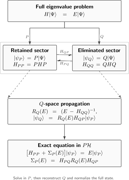
Projection does not simply erase $Q$. The resolvent $R_Q(E)=(E-H_{QQ})^{-1}$ propagates an amplitude through the eliminated sector. Returning to $P$ produces the self-energy $\Sigma_P(E)$, while the same excursion reconstructs $\lvert\psi_Q\rangle$.

Exact Elimination and the Schur Complement

Suppose $E-H_{QQ}$ is invertible on $Q\mathcal H$. Define the eliminated-space resolvent

$$R_Q(E) = \left( E-H_{QQ} \right)^{-1}.$$

The second block equation can be solved exactly:

$$\lvert\psi_Q\rangle = R_Q(E) H_{QP}\lvert\psi_P\rangle.$$

Substitution into the first block equation gives

$$H_{\mathrm{eff}}(E) \lvert\psi_P\rangle = E\lvert\psi_P\rangle,$$

where

$$\begin{aligned} H_{\mathrm{eff}}(E) &= H_{PP} + \Sigma_P(E), \\ \Sigma_P(E) &= H_{PQ} R_Q(E) H_{QP}. \end{aligned}$$

The self-energy $\Sigma_P(E)$ represents the ordered process

$$P \xrightarrow{\,H_{QP}\,} Q \xrightarrow{\,R_Q(E)\,} Q \xrightarrow{\,H_{PQ}\,} P.$$

It contains every repeated interaction internal to $H_{QQ}$ because the resolvent is exact. The formula therefore does not assume weak $P$–$Q$ coupling. It does, however, replace a linear eigenvalue problem on the full Hilbert space with a generally nonlinear eigenvalue problem on $P\mathcal H$, because the operator being diagonalized depends on the unknown $E$.

Determinant identity

In finite dimensions the same reduction is the Schur complement of $E-H_{QQ}$. Wherever this block is invertible,

$$\begin{aligned} \det(EI-H) &= \det(EI_Q-H_{QQ}) \\ &\quad\times \det\!\left( EI_P-H_{\mathrm{eff}}(E) \right). \end{aligned}$$

Thus the reduced secular equation reproduces the full eigenvalues that have nonzero projection into $P$. The apparent poles in $H_{\mathrm{eff}}(E)$ are essential: when the factors are multiplied, pole-zero cancellations recover the polynomial characteristic equation of the full matrix.

An eigenstate lying entirely in $Q\mathcal H$ has $\lvert\psi_P\rangle=0$ and is not represented by a nonzero solution of the reduced equation. This is expected. A projection method preserves information seen by the chosen model space; it does not promise to expose states orthogonal to it.

The Projected Resolvent

Projection can reduce the resolvent itself, not only individual eigenvectors. Let

$$G(z) = \left( z-H \right)^{-1},$$

with $z$ outside the spectra needed to define the inverses. The $P$ block obeys

$$PG(z)P = \left[ z-H_{\mathrm{eff}}(z) \right]^{-1},$$

where

$$H_{\mathrm{eff}}(z) = H_{PP} + H_{PQ} \left( z-H_{QQ} \right)^{-1} H_{QP}.$$

This identity explains why an energy-dependent effective Hamiltonian can reproduce projected spectral poles and response functions exactly. It also shows what it is designed to match: the $P$-space Green function, not necessarily a globally defined, energy-independent operator on the full Hilbert space. The Resolvent Operator page develops the spectral and analytic meaning of $G(z)$.

Reconstructing States and Their Norms

Solving the reduced equation is only half of the construction. The eliminated component is

$$\lvert\psi_Q\rangle = R_Q(E) H_{QP}\lvert\psi_P\rangle,$$

so the full eigenstate is

$$\lvert\Psi\rangle = \left[ P + R_Q(E)H_{QP} \right] \lvert\psi_P\rangle.$$

For a real bound-state energy outside the spectrum of $H_{QQ}$, the resolvent is self-adjoint. Differentiating the effective Hamiltonian gives

$$\frac{\partial H_{\mathrm{eff}}}{\partial E} = - H_{PQ} R_Q(E)^2 H_{QP}.$$

Consequently,

$$\begin{aligned} \langle\Psi\vert\Psi\rangle &= \langle\psi_P\vert\psi_P\rangle + \langle\psi_Q\vert\psi_Q\rangle \\ &= \left\langle\psi_P\left| I_P - \frac{\partial H_{\mathrm{eff}}}{\partial E} \right|\psi_P\right\rangle. \end{aligned}$$

The projected eigenvector should therefore not generally be normalized as though it were the full state. If a solution direction $\lvert\widehat\psi_P\rangle$ has unit norm inside $P$, the probability carried by the retained sector after full normalization is

$$Z_P = \left[ \left\langle\widehat\psi_P\left| I_P - \frac{\partial H_{\mathrm{eff}}}{\partial E} \right|\widehat\psi_P\right\rangle \right]^{-1}.$$

Because $-\partial_EH_{\mathrm{eff}}$ is positive semidefinite in this bound-state setting, $0\lt Z_P\le1$.

Observables also need reconstruction

Define the energy-dependent embedding on the model space by

$$\Omega(E) = P + R_Q(E)H_{QP}.$$

Then $\lvert\Psi\rangle=\Omega(E)\lvert\psi_P\rangle$. For an observable $O$, its exact reduced matrix element is built from

$$O_{\mathrm{eff}}(E) = \Omega(E)^\dagger O \Omega(E),$$

together with the norm operator

$$N(E) = \Omega(E)^\dagger\Omega(E) = I_P - \frac{\partial H_{\mathrm{eff}}}{\partial E}.$$

For one reconstructed state,

$$\langle O\rangle = \frac{ \langle\psi_P\vert O_{\mathrm{eff}}(E) \vert\psi_P\rangle }{ \langle\psi_P\vert N(E) \vert\psi_P\rangle }.$$

Using $H_{\mathrm{eff}}$ while replacing every observable by $POP$ omits the same virtual admixtures that generated the effective Hamiltonian. In a Schrieffer–Wolff treatment this information appears as the unitary dressing of states and observables.

Worked Example: One Retained Level

Consider

$$H = \begin{pmatrix} \varepsilon_p & g \\ g^* & \varepsilon_q \end{pmatrix},$$

and retain the first basis state. Then

$$H_{\mathrm{eff}}(E) = \varepsilon_p + \frac{\lvert g\rvert^2} {E-\varepsilon_q}.$$

The reduced eigenvalue equation is

$$E = \varepsilon_p + \frac{\lvert g\rvert^2} {E-\varepsilon_q}.$$

Multiplying by $E-\varepsilon_q$ gives

$$(E-\varepsilon_p) (E-\varepsilon_q) - \lvert g\rvert^2 = 0,$$

with exact roots

$$E_\pm = \frac{\varepsilon_p+\varepsilon_q}{2} \pm \sqrt{ \left( \frac{\varepsilon_p-\varepsilon_q}{2} \right)^2 + \lvert g\rvert^2 }.$$

The eliminated amplitude satisfies

$$\frac{\psi_q}{\psi_p} = \frac{g^*} {E-\varepsilon_q}.$$

If the projected component is initially assigned unit norm, the retained probability in the normalized full eigenstate is

$$Z_P(E) = \left[ 1 + \frac{\lvert g\rvert^2} {(E-\varepsilon_q)^2} \right]^{-1}.$$

This agrees with the derivative formula because

$$\frac{\partial H_{\mathrm{eff}}}{\partial E} = - \frac{\lvert g\rvert^2} {(E-\varepsilon_q)^2}.$$

Let $d=\varepsilon_p-\varepsilon_q$ and suppose $\lvert g/d\rvert\ll1$. The root connected continuously to $\varepsilon_p$ is

$$E_p = \varepsilon_p + \frac{\lvert g\rvert^2}{d} - \frac{\lvert g\rvert^4}{d^3} + O\!\left( \frac{\lvert g\rvert^6}{d^5} \right).$$

The familiar second-order energy denominator is therefore the first approximation to an exact energy-dependent equation. Near $d=0$, the expansion fails while the exact square root remains regular and produces an avoided crossing.

Worked Example: An Induced Coupling

Let two retained states couple to one remote state:

$$H = \begin{pmatrix} \varepsilon_1 & 0 & g_1^* \\ 0 & \varepsilon_2 & g_2^* \\ g_1 & g_2 & \Delta \end{pmatrix}.$$

Choose $P$ to retain the first two basis states and $Q$ to retain the third. Exact elimination gives

$$\begin{aligned} H_{\mathrm{eff}}(E) &= \begin{pmatrix} \varepsilon_1 & 0 \\ 0 & \varepsilon_2 \end{pmatrix} \\ &\quad+ \frac{1}{E-\Delta} \begin{pmatrix} \lvert g_1\rvert^2 & g_1^*g_2 \\ g_2^*g_1 & \lvert g_2\rvert^2 \end{pmatrix}. \end{aligned}$$

Even though the retained states have no direct matrix element, the eliminated state mediates one. If

$$\lvert E\rvert, \lvert\varepsilon_1\rvert, \lvert\varepsilon_2\rvert \ll \lvert\Delta\rvert,$$

freezing the denominator at $E=0$ gives

$$\begin{aligned} H_{\mathrm{eff}} &\simeq \begin{pmatrix} \varepsilon_1 & 0 \\ 0 & \varepsilon_2 \end{pmatrix} \\ &\quad- \frac{1}{\Delta} \begin{pmatrix} \lvert g_1\rvert^2 & g_1^*g_2 \\ g_2^*g_1 & \lvert g_2\rvert^2 \end{pmatrix}. \end{aligned}$$

The diagonal entries are virtual level shifts. The off-diagonal entries are an induced interaction of order $g_1^*g_2/\Delta$.

For $\varepsilon_1=\varepsilon_2=0$, the vector

$$\lvert D\rangle \propto g_2\lvert1\rangle - g_1\lvert2\rangle$$

is annihilated by $H_{QP}$ and is therefore an exact dark eigenstate with energy zero. The orthogonal bright combination couples to $Q$ and is shifted. Projection makes the distinction transparent: only the component that can leave $P$ acquires the self-energy.

From Exact Elimination to an Approximation

The exact expression can be expanded around a reference energy $E_0$. Write

$$R_0 = \left( E_0-H_{QQ} \right)^{-1}.$$

If

$$\lvert E-E_0\rvert \lVert R_0\rVert \lt1,$$

the resolvent has the convergent Neumann expansion

$$\begin{aligned} R_Q(E) &= R_0 - (E-E_0)R_0^2 \\ &\quad+ (E-E_0)^2R_0^3 - \cdots. \end{aligned}$$

Keeping only $R_0$ yields the static approximation

$$H_{\mathrm{eff}} \simeq H_{PP} + H_{PQ}R_0H_{QP}.$$

If the off-diagonal coupling has scale $v$ and the eliminated spectrum is separated by a scale $\Delta$, then

$$\lVert\Sigma_P\rVert \sim \frac{v^2}{\Delta}.$$

The neglected energy dependence is smaller only when the retained energy window is also narrow compared with $\Delta$. Weak coupling and a narrow model-space window are related but distinct conditions.

This expansion connects several methods:

• Brillouin–Wigner Perturbation Theory keeps an energy-dependent effective equation and solves it self-consistently.
• Folded Effective Hamiltonians reorganizes Q-box energy dependence into one energy-independent model-space interaction.
• Quasi-Degenerate Perturbation Theory retains a cluster of close levels and constructs a Hermitian model-space matrix order by order.
• Schrieffer–Wolff Transformation uses a perturbative unitary transformation to produce an energy-independent block Hamiltonian and dressed observables.
• Adiabatic Elimination turns the exact time-domain memory equation into a local slow generator when the eliminated response is fast.

These are not competing names for one formula. They preserve different structures and organize the same virtual processes in different ways.

Resolvent Distance and Error Control

For self-adjoint $H_{QQ}$ and real $E$ outside its spectrum,

$$\lVert R_Q(E)\rVert = \frac{1}{ \operatorname{dist} \left( E,\operatorname{spec}H_{QQ} \right) }.$$

Therefore

$$\lVert\Sigma_P(E)\rVert \le \frac{ \lVert H_{PQ}\rVert \lVert H_{QP}\rVert }{ \operatorname{dist} \left( E,\operatorname{spec}H_{QQ} \right) }.$$

For a self-adjoint $H$, the numerator is $\lVert H_{PQ}\rVert^2$. This estimate captures the small-denominator problem directly. As $E$ approaches the eliminated spectrum, the resolvent grows, the reconstructed $Q$ weight grows, and a low-order static approximation loses control.

For the expansion around $E_0$, the resolvent identity gives the explicit bound

$$\begin{aligned} \lVert R_Q(E)-R_0\rVert &\le \frac{ \lvert E-E_0\rvert \lVert R_0\rVert^2 }{ 1- \lvert E-E_0\rvert \lVert R_0\rVert }. \end{aligned}$$

Multiplying by the norms of $H_{PQ}$ and $H_{QP}$ bounds the error made by freezing the self-energy. Small Parameters and Error Estimates develops the broader discipline of turning such ratios into honest validity statements.

Relation to Scattering

In a discrete bound-state problem, $E$ may lie outside the spectrum of $H_{QQ}$. In scattering, $Q\mathcal H$ can contain a continuum at the physical energy. The resolvent is then specified by a boundary value such as

$$R_Q(E^+) = \left( E+i0-H_{QQ} \right)^{-1}.$$

Formally,

$$R_Q(E^+) = \mathcal P \frac{1}{E-H_{QQ}} - i\pi\delta(E-H_{QQ}).$$

The self-energy consequently has a real dispersive part and, for open eliminated channels, a negative imaginary part:

$$\Sigma_P(E^+) = \Delta_P(E) - \frac{i}{2}\Gamma_P(E).$$

The width operator

$$\Gamma_P(E) = 2\pi H_{PQ} \delta(E-H_{QQ}) H_{QP}$$

is positive semidefinite. It describes probability leaving the retained channel while the full closed-system evolution remains unitary. Thresholds, analytic continuation, resonance poles, and optical potentials are developed at their canonical home, Feshbach Projection Formalism.

Method Guide

Question	Natural construction	Character of the result
What is the exact equation seen by a chosen finite model space?	P/Q projection and Schur complement	Energy dependent; exact where the resolvent exists
How do open channels shift and broaden retained states?	Feshbach projection	Boundary-value resolvent; generally non-Hermitian in $P$
How should several close levels be treated together?	Quasi-degenerate perturbation theory	Hermitian model-space matrix order by order
How can a separated block be decoupled perturbatively?	Schrieffer–Wolff transformation	Energy-independent unitary block diagonalization
How can one iterate an energy-dependent perturbative equation?	Brillouin–Wigner perturbation theory	Nonlinear eigenvalue problem

The best method is fixed by the desired output. A projected Green function, a reusable low-energy Hamiltonian, and a perturbative spectrum are related objects, but they are not interchangeable without matching states and observables.

Domain and Numerical Caveats

The finite-dimensional algebra extends to operators on infinite-dimensional Hilbert spaces only with additional care. For an unbounded Hamiltonian:

• $P$ and $Q$ must act compatibly with the relevant operator domains;
• the inverse of $E-H_{QQ}$ must exist on the vectors to which it is applied;
• continuum energies require boundary values rather than ordinary bounded inverses;
• norm estimates may need relative-boundedness or quadratic-form arguments.

Numerically, projection is useful only if applying $R_Q(E)$ is cheaper than solving the full problem. One may never form the inverse explicitly; instead, solve the linear system

$$\left( E-H_{QQ} \right)\lvert x\rangle = H_{QP}\lvert\psi_P\rangle.$$

For large sparse problems, this avoids a dense inverse and lets iterative linear solvers exploit the structure of $H_{QQ}$. Near a pole, however, that linear system becomes ill-conditioned, faithfully signaling that the chosen reduction is difficult.

Common Mistakes

• Calling $H_{PP}$ the effective Hamiltonian without accounting for virtual excursions through $Q$.
• Treating the exact elimination formula as though it already were a weak-coupling expansion.
• Forgetting that $H_{\mathrm{eff}}(E)$ defines a nonlinear eigenvalue problem.
• Normalizing $\lvert\psi_P\rangle$ as the full state and ignoring the reconstructed $Q$ weight.
• Computing observables with $POP$ while retaining self-energy corrections in the Hamiltonian.
• Freezing the resolvent at $E_0$ without checking the width of the retained energy window.
• Eliminating a state whose energy is close to the energies being sought.
• Interpreting a non-Hermitian projected scattering operator as nonunitarity of the full closed system.
• Using a matrix inverse explicitly when a structured linear solve is more stable.

Exercises

1. Derive the block equations

Starting from $H\lvert\Psi\rangle=E\lvert\Psi\rangle$, derive the two coupled block equations. Show that $[P,H]=0$ implies that $P\mathcal H$ and $Q\mathcal H$ evolve independently.

Solution

Insert $I=P+Q$ on the state and act first with $P$:

$$\begin{aligned} PH(P+Q)\lvert\Psi\rangle &= EP\lvert\Psi\rangle, \\ H_{PP}\lvert\psi_P\rangle + H_{PQ}\lvert\psi_Q\rangle &= E\lvert\psi_P\rangle. \end{aligned}$$

Acting with $Q$ similarly gives

$$H_{QP}\lvert\psi_P\rangle + H_{QQ}\lvert\psi_Q\rangle = E\lvert\psi_Q\rangle.$$

If $[P,H]=0$, then

$$\begin{aligned} PHQ &= PH(I-P) \\ &= PH-PHP \\ &= 0, \end{aligned}$$

and similarly $QHP=0$. The off-diagonal blocks vanish, so each component satisfies its own equation and no amplitude is transferred between the sectors.

2. Prove the determinant factorization

For a finite-dimensional matrix, use block Gaussian elimination to prove

$$\begin{aligned} \det(EI-H) &= \det(EI_Q-H_{QQ}) \\ &\quad\times \det(EI_P-H_{\mathrm{eff}}(E)). \end{aligned}$$

Solution

Write

$$EI-H = \begin{pmatrix} E-H_{PP} & -H_{PQ} \\ -H_{QP} & E-H_{QQ} \end{pmatrix}.$$

Left-multiply by the block triangular matrix

$$L = \begin{pmatrix} I_P & H_{PQ}(E-H_{QQ})^{-1} \\ 0 & I_Q \end{pmatrix},$$

whose determinant is one. Define

$$S_P(E) = E-H_{\mathrm{eff}}(E).$$

Direct multiplication gives

$$L(EI-H) = \begin{pmatrix} S_P(E) & 0 \\ -H_{QP} & E-H_{QQ} \end{pmatrix}.$$

The determinant of the resulting block triangular matrix is the product of the two diagonal-block determinants, proving the identity.

3. Check the two-level normalization

For the two-level model, reconstruct the eliminated amplitude and verify both the direct norm formula and the derivative formula for $Z_P(E)$.

Solution

The $Q$ equation gives

$$\psi_q = \frac{g^*}{E-\varepsilon_q} \psi_p.$$

Taking $\psi_p=1$ temporarily,

$$\lVert\Psi\rVert^2 = 1 + \frac{\lvert g\rvert^2} {(E-\varepsilon_q)^2}.$$

The normalized $P$ weight is therefore

$$Z_P(E) = \left[ 1 + \frac{\lvert g\rvert^2} {(E-\varepsilon_q)^2} \right]^{-1}.$$

On the other hand,

$$\partial_EH_{\mathrm{eff}}(E) = - \frac{\lvert g\rvert^2} {(E-\varepsilon_q)^2},$$

so

$$Z_P(E) = \left[ 1-\partial_EH_{\mathrm{eff}}(E) \right]^{-1}.$$

The two calculations agree.

4. Find the dark and bright combinations

Set $\varepsilon_1=\varepsilon_2=0$ in the three-level example. Find one normalized state in $P$ that does not couple to $Q$, and identify the orthogonal bright direction.

Solution

For a retained vector with amplitudes $(c_1,c_2)$,

$$H_{QP} \begin{pmatrix} c_1\\c_2 \end{pmatrix} = g_1c_1+g_2c_2.$$

Choosing $(c_1,c_2)=(g_2,-g_1)$ makes this expression vanish. Thus

$$\lvert D\rangle = \frac{ g_2\lvert1\rangle-g_1\lvert2\rangle }{ \sqrt{\lvert g_1\rvert^2+\lvert g_2\rvert^2} }$$

is dark and has no $Q$ component. An orthogonal normalized bright direction is

$$\lvert B\rangle = \frac{ g_1^*\lvert1\rangle+g_2^*\lvert2\rangle }{ \sqrt{\lvert g_1\rvert^2+\lvert g_2\rvert^2} }.$$

Only $\lvert B\rangle$ is acted on by the rank-one self-energy. Its leading far-detuned shift is

$$\delta E_B \simeq - \frac{ \lvert g_1\rvert^2+\lvert g_2\rvert^2 }{\Delta}.$$

5. Bound the frozen-resolvent error

Let $\delta=E-E_0$ and assume $\lvert\delta\rvert\lVert R_0\rVert\lt1$. Derive a norm bound on $R_Q(E)-R_0$ and hence on the error in the frozen self-energy.

Solution

Since

$$R_Q(E) = \left( I+\delta R_0 \right)^{-1} R_0,$$

the resolvent identity gives

$$R_Q(E)-R_0 = - \delta R_0^2 \left( I+\delta R_0 \right)^{-1}.$$

The Neumann-series estimate is

$$\left\lVert \left( I+\delta R_0 \right)^{-1} \right\rVert \le \frac{1}{ 1-\lvert\delta\rvert\lVert R_0\rVert }.$$

Therefore

$$\lVert R_Q(E)-R_0\rVert \le \frac{ \lvert\delta\rvert\lVert R_0\rVert^2 }{ 1-\lvert\delta\rvert\lVert R_0\rVert }.$$

Multiplying on the left and right gives

$$\begin{aligned} \lVert \Sigma_P(E)-\Sigma_P(E_0) \rVert &\le \lVert H_{PQ}\rVert \lVert H_{QP}\rVert \\ &\quad\times \frac{ \lvert\delta\rvert\lVert R_0\rVert^2 }{ 1-\lvert\delta\rvert\lVert R_0\rVert }. \end{aligned}$$

6. Show that the scattering width is positive

Assume the spectral delta operator $\delta(E-H_{QQ})$ is positive. Show that $\Gamma_P(E)$ is positive semidefinite.

Solution

For any $\lvert\phi_P\rangle$, define

$$\lvert\chi_Q\rangle = H_{QP}\lvert\phi_P\rangle.$$

For compactness, also write

$$D_Q(E) = \delta(E-H_{QQ}).$$

Then

$$\begin{aligned} \gamma_\phi(E) &\equiv \langle\phi_P\vert \Gamma_P(E) \vert\phi_P\rangle, \\ \gamma_\phi(E) &= 2\pi \langle\chi_Q\vert D_Q(E) \vert\chi_Q\rangle \\ &= 2\pi \left\lVert D_Q(E)^{1/2} \lvert\chi_Q\rangle \right\rVert^2 \\ &\ge0. \end{aligned}$$

Thus the imaginary part of the outgoing self-energy is $-\Gamma_P/2$ with a nonnegative width. The sign encodes loss from the retained channel into outgoing eliminated channels.

Cross-Links

• Effective Hamiltonians and Scale Separation
• Projectors
• Resolvent Operator
• Brillouin–Wigner Perturbation Theory
• Folded Effective Hamiltonians
• Adiabatic Elimination
• Quasi-Degenerate Perturbation Theory
• Feshbach Projection Formalism
• Schrieffer–Wolff Transformation
• Matrix Diagonalization

References

1. P.-O. Löwdin, “A note on the quantum-mechanical perturbation theory,” The Journal of Chemical Physics 19, 1396–1401 (1951) — the original partitioning treatment of two classes of approximate states.
2. H. Feshbach, “Unified theory of nuclear reactions,” Annals of Physics 5, 357–390 (1958).
3. H. Feshbach, “A unified theory of nuclear reactions. II,” Annals of Physics 19, 287–313 (1962).
4. C. Bloch, “Sur la théorie des perturbations des états liés,” Nuclear Physics 6, 329–347 (1958).
5. R. A. Horn and C. R. Johnson, Matrix Analysis, 2nd ed., Cambridge University Press (2013) — block matrices and Schur complements.
6. T. Kato, Perturbation Theory for Linear Operators, 2nd ed., Springer (1976; corrected printing 1995) — operator and spectral foundations.
7. E. N. Economou, Green’s Functions in Quantum Physics, 3rd ed., Springer (2006) — resolvents, self-energies, and projected Green functions.
8. C. Cohen-Tannoudji, B. Diu, and F. Laloë, Quantum Mechanics, Vol. 2, Wiley (1977) — projection operators and effective Hamiltonians in perturbation theory.
9. S. Bravyi, D. P. DiVincenzo, and D. Loss, “Schrieffer–Wolff transformation for quantum many-body systems,” Annals of Physics 326, 2793–2826 (2011) — comparison with unitary low-energy reduction.