Effective Hamiltonians in Many-Body Systems

An effective Hamiltonian acts in a deliberately retained subspace and reproduces specified low-energy predictions of a more detailed parent Hamiltonian to a declared accuracy. High-energy states are not simply forgotten. Virtual excursions through them generate energy shifts, exchange interactions, constrained hopping, potential scattering, multispin terms, and corrections to observables.

The central structure is

$$\text{low-energy state} \longrightarrow \text{virtual high-energy state} \longrightarrow \text{low-energy state}.$$

If the coupling for each step is $v$ and the intermediate-state cost is $\Delta$, the induced scale is typically

$$\frac{v^2}{\Delta}.$$

This estimate is only a beginning. A trustworthy reduction must specify:

• the parent Hamiltonian and all sign conventions;
• the retained projector $P$ and eliminated projector $Q$;
• the gap or energy denominators separating the sectors;
• the order and local parameter of the expansion;
• every generated operator retained or discarded;
• the energy, temperature, frequency, and filling window of use;
• the transformation of states and observables;
• the benchmark used to test the truncation.

Merely replacing $H$ by $PHP$ is generally not enough. That replacement keeps processes that never leave the model space but misses the virtual processes responsible for superexchange and Kondo exchange.

Canonical Scope

This page is the canonical many-body treatment of:

• projected low-energy sectors in extensive Hilbert spaces;
• the local meaning of a Schrieffer–Wolff expansion;
• virtual paths and their energy denominators;
• the large-$U$ Hubbard-to-Heisenberg reduction;
• why doping produces projected hopping and the t–J structure instead of a pure spin model;
• the Anderson-to-Kondo reduction as a comparative preview;
• constants, density terms, potential scattering, three-site terms, and higher-order interactions;
• locality, symmetry, internal unitary freedom, and thermodynamic scaling;
• effective states and observables;
• validation and breakdown tests.

Neighboring pages retain separate ownership:

• Emergence and Effective Degrees of Freedom owns the cross-mechanism audit of variable selection, observable matching, error, and breakdown; this page retains controlled projection, Schrieffer–Wolff reductions, generated operators, and dressed observables.
• Projection Methods owns exact $P/Q$ block elimination, energy-dependent Schur complements, projected resolvents, and state reconstruction.
• Schrieffer–Wolff Transformation owns the general unitary generator, commutator expansion, and method-level comparison with Feshbach and folded Hamiltonians.
• Effective Hamiltonians in Quantum Matter owns the exact Hubbard-dimer benchmark and band effective-mass application.
• Renormalization Group Preview owns scale-by-scale coarse graining and coupling-space flow; projection here instead selects a retained model space across an explicit energy separation.
• Quasiparticles Overview owns effective Hamiltonians written in terms of emergent particle-like branches; this page owns how controlled projection derives a retained Hamiltonian and its dressed observables.
• Hubbard Model and Heisenberg Model own the definitions and physics of those models. The Anderson Impurity Model dossier owns the compact charge-fluctuating impurity specification, limits, and finite benchmark; Anderson Impurity Model Preview owns its detailed spectra, thermodynamics, and DMFT physics. The Kondo Model dossier owns the compact spin-model specification, limits, and finite benchmark; the Kondo Model Preview owns its detailed scaling and screening physics.
• Common Many-Body Hamiltonians remains the compact formula sheet.

The goal here is not to solve the resulting low-energy model. It is to derive what that model is, state what was removed, and identify when the reduction can be trusted.

Retained and Eliminated Sectors

Let

$$P+Q=I, \qquad P^2=P, \qquad Q^2=Q, \qquad PQ=0.$$

The model space is $P\mathcal H$. The eliminated space is $Q\mathcal H$. Write

$$H=H_0+V,$$

where $H_0$ preserves both sectors:

$$[H_0,P]=0.$$

It is useful to split the perturbation into block-diagonal and block-off-diagonal pieces:

$$\begin{aligned} V_{\mathrm d} &= PVP+QVQ, \\ V_{\mathrm{od}} &= PVQ+QVP. \end{aligned}$$

$V_{\mathrm d}$ acts without changing sector. $V_{\mathrm{od}}$ creates or removes the high-energy configurations that will appear virtually.

The gap is between sectors

Suppose the retained manifold has reference energy $E_0$ and

$$Q(H_0-E_0)Q \ge \Delta Q, \qquad \Delta>0.$$

This does not require $P\mathcal H$ to be internally gapped. A half-filled Mott system can have a charge gap of order $U$ between $P$ and $Q$ while its retained spin sector is gapless in the thermodynamic limit.

The projection controls excursions across the sector gap. It does not solve infrared dynamics inside the retained sector.

Projectors encode physical assumptions

Examples include:

Parent problem	Retained sector $P$	Eliminated sector $Q$
half-filled large-$U$ Hubbard model	one fermion per site	states with doublon–hole pairs
doped large-$U$ Hubbard model	no double occupancy, holes allowed	states with at least one doublon
Anderson impurity in local-moment regime	singly occupied impurity doublet	empty and doubly occupied impurity
crystal-field multiplet	selected low multiplet	higher local multiplets
multiband lattice model	active bands or orbitals	remote bands or orbitals

A projector is not justified merely because its states are intuitively interesting. The omitted sector must remain sufficiently costly over the parameter and kinematic range of interest.

Second-Order Effective Hamiltonian

For a degenerate retained manifold at $E_0$, the leading energy-independent result is

$$\begin{aligned} H_{\mathrm{eff}} ={}& E_0P + PVP \\ &- PVQ \left[ Q(H_0-E_0)Q \right]^{-1} QVP \\ &+ O\!\left( \frac{V^3}{\Delta^2} \right). \end{aligned}$$

The inverse acts only in $Q\mathcal H$. The second-order term has the path structure

$$P \xrightarrow{\ V\ } Q \xrightarrow{\ V\ } P.$$

For retained states $\lvert a\rangle$ and $\lvert b\rangle$ with a common energy $E_0$,

$$\langle a| H_{\mathrm{eff}}^{(2)} |b\rangle = \sum_{m\in Q} \frac{ \langle a|V|m\rangle \langle m|V|b\rangle }{ E_0-E_m }.$$

Every allowed intermediate state contributes. Relative phases, fermionic signs, spin selection rules, and unequal denominators can make virtual paths add or cancel.

Quasi-degenerate retained states

If $\lvert a\rangle$ and $\lvert b\rangle$ have nearby but unequal unperturbed energies, a standard Hermitian second-order form is

$$\begin{aligned} \langle a| H_{\mathrm{eff}}^{(2)} |b\rangle ={}& \frac12 \sum_{m\in Q} \langle a|V|m\rangle \langle m|V|b\rangle \\ &\times \left[ \frac1{E_a-E_m} + \frac1{E_b-E_m} \right]. \end{aligned}$$

This is one consistent convention. Bloch, Löwdin, Van Vleck, Brillouin–Wigner, and Schrieffer–Wolff effective Hamiltonians can differ off shell or by a unitary transformation inside $P$. Their coefficients should not be mixed term by term.

Quasi-Degenerate Perturbation Theory owns the general model-space treatment.

Schrieffer–Wolff View

Choose an anti-Hermitian generator

$$S^\dagger=-S$$

and transform

$$\widetilde H = e^SHe^{-S}.$$

The generator is chosen so that

$$P\widetilde H Q = 0$$

through the desired order. With $S=S_1+O(V^2)$, a convenient first-order convention is

$$[H_0,S_1] = V_{\mathrm{od}}.$$

Then the retained block through second order is

$$\begin{aligned} H_{\mathrm{eff}} ={}& P\widetilde H P \\ ={}& P(H_0+V_{\mathrm d})P + \frac12 P[S_1,V_{\mathrm{od}}]P + O(V^3). \end{aligned}$$

The projected-resolvent and Schrieffer–Wolff forms organize the same virtual physics differently. The unitary form has an important advantage: it also tells us how to transform states and observables.

The detailed construction, including sign conventions for $S$, belongs to Schrieffer–Wolff Transformation.

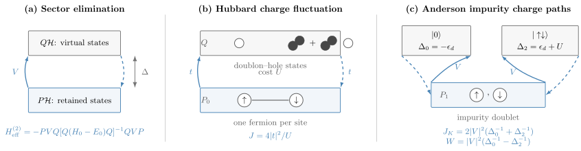
Virtual-state grammar for two canonical reductions. The Hubbard model has one dominant charge cost $U$ in the simplest limit and produces $J=4|t|^2/U$. The Anderson impurity has two charge costs, $\Delta_0=-\epsilon_d$ and $\Delta_2=\epsilon_d+U$; their exchange amplitudes add, while their potential-scattering amplitudes subtract.

Why Many-Body Control Is Local

For an $L$-site lattice, the norm of the total perturbation often scales with $L$. A condition such as

$$\frac{\lVert V\rVert}{\Delta} \ll1$$

can therefore fail even when every local virtual process is weak. The useful control parameter is instead built from local matrix elements, gaps, coordination, and connected clusters.

For local coupling scale $v$ and coordination $z$, a rough diagnostic is

$$\epsilon_{\mathrm{loc}} \sim \frac{zv}{\Delta}.$$

This is not a universal theorem. It reminds us that one site can access several virtual channels. The actual coefficient depends on geometry, operator norms, statistics, and cancellations.

Linked support

At order $n$, a local perturbation can generate operators supported on connected clusters reached by $n$ elementary couplings. Thus:

• second order commonly generates bond exchange or correlated hopping;
• third order can detect triangular loops or complex hopping phases;
• fourth order can generate longer-range exchange and four-site ring exchange;
• operator range and body order generally grow with perturbative order.

Disconnected virtual processes contribute to extensive constants or factorized pieces. A linked-cluster organization is what keeps local effective interactions meaningful in the thermodynamic limit.

Energy density versus whole-spectrum accuracy

A truncated local Hamiltonian can approximate low-energy densities and local dynamics even though it does not approximate every eigenvalue of the exponentially large spectrum. Claims of control must name the quantity:

• ground-state energy density;
• a low-energy band of states;
• local observables for finite times;
• thermal observables below a cutoff;
• matrix elements within a symmetry sector.

“The effective Hamiltonian is accurate” is incomplete without this target.

Hubbard to Heisenberg

Consider the repulsive single-band Hubbard Hamiltonian

$$H = H_U+T,$$

with

$$H_U = U \sum_i n_{i\uparrow}n_{i\downarrow}, \qquad U>0,$$

and

$$T = - \sum_{\langle i,j\rangle,\sigma} \left( t_{ij} c_{i\sigma}^\dagger c_{j\sigma} + t_{ij}^* c_{j\sigma}^\dagger c_{i\sigma} \right).$$

Hubbard Model owns the complete model definition, symmetry conventions, limiting cases, and observables.

Half filling and the no-doublon sector

At one fermion per site, let $P_0$ project onto states with no double occupancy. With the total particle number fixed to the number of sites, every retained site is singly occupied.

A single hop necessarily creates one doublon and one hole, so

$$P_0TP_0 = 0.$$

The first nonzero dynamics is second order:

$$H_{\mathrm{eff}}^{(2)} = - P_0TQ \frac1{QH_UQ} QTP_0.$$

For the simplest uniform model, the relevant intermediate states cost $U$, giving

$$H_{\mathrm{eff}}^{(2)} = - \frac1U P_0TQT P_0.$$

One bond fixes the exchange

On a bond $\langle i,j\rangle$, define the dimensionless spin operator

$$\mathbf s_i = \frac12 \sum_{\alpha,\beta} c_{i\alpha}^\dagger \boldsymbol\sigma_{\alpha\beta} c_{i\beta}.$$

The singlet projector for two singly occupied sites is

$$P_{S,ij} = \frac14 - \mathbf s_i\cdot\mathbf s_j.$$

The spin singlet couples to the two virtual doublon–hole configurations. Fermionic antisymmetry makes the corresponding triplet amplitudes vanish or cancel. The shifts are

$$\Delta E_S = - \frac{4|t_{ij}|^2}{U}, \qquad \Delta E_T = 0.$$

Therefore the bond operator is

$$\begin{aligned} H_{ij}^{(2)} &= -J_{ij}P_{S,ij} \\ &= J_{ij} \left( \mathbf s_i\cdot\mathbf s_j - \frac14 \right), \end{aligned}$$

with

$$J_{ij} = \frac{4|t_{ij}|^2}{U} >0.$$

Positive $J_{ij}$ is antiferromagnetic in this convention. The exact dimer matrix, singlet–triplet spectrum, and finite-$t/U$ benchmark belong to Effective Hamiltonians in Quantum Matter.

Lattice Hamiltonian

Summing bond contributions gives

$$H_{\mathrm{spin}} = \sum_{\langle i,j\rangle} J_{ij} \left( \mathbf s_i\cdot\mathbf s_j - \frac14 \right) + \delta H.$$

At fixed half filling, the constant $-J_{ij}/4$ per bond can be dropped when only state differences and dynamics are needed. The remaining operator is the antiferromagnetic Heisenberg model.

The hierarchy of scales is

$$J \sim \frac{t^2}{U} \ll |t| \ll U.$$

Charge excitations become costly at scale $U$, while spin dynamics survives at the parametrically smaller scale $J$. A system can therefore display well-formed local moments at temperatures below $U$ but still remain thermally disordered relative to $J$.

Virtual does not mean absent

The block-diagonal low-energy state has no doublon by construction. The physical state is

$$|\Psi\rangle = e^{-S} |\Psi_{\mathrm{eff}}\rangle.$$

Its doublon–hole amplitude is generally

$$O\!\left( \frac{t}{U} \right),$$

so its double-occupancy probability is

$$O\!\left( \frac{t^2}{U^2} \right).$$

The spin Hamiltonian freezes real low-energy charge motion at half filling; it does not claim that the parent Hubbard eigenstate has exactly zero virtual charge fluctuation.

Away from Half Filling

With holes present, a fermion can hop into an empty site without creating a doublon. Consequently,

$$P_0TP_0 \ne 0.$$

Define projected fermion operators

$$\widetilde c_{i\sigma} = P_0c_{i\sigma}P_0 = c_{i\sigma} \left( 1-n_{i\bar\sigma} \right)$$

within the no-doublon Hilbert space. The leading strong-coupling Hamiltonian has the structure

$$\begin{aligned} H_{t\text{–}J} ={}& - \sum_{\langle i,j\rangle,\sigma} \left( t_{ij} \widetilde c_{i\sigma}^\dagger \widetilde c_{j\sigma} + \mathrm{h.c.} \right) \\ &+ \sum_{\langle i,j\rangle} J_{ij} \left( \mathbf s_i\cdot\mathbf s_j - \frac14 n_in_j \right) \\ &+ H_{\mathrm{3site}} + \cdots. \end{aligned}$$

The projected hopping is first order in $t$. Exchange and three-site correlated hopping are second order in $t/U$. Omitting $H_{\mathrm{3site}}$ defines an additional approximation; it is not part of the projection identity.

t–J Model Preview owns the constrained Hilbert space, projected-operator algebra, model physics, and variants.

Why the density term matters

At half filling, $n_in_j=1$ on every retained bond, so

$$-\frac14J_{ij}n_in_j$$

is a constant. With holes, it depends on configuration and cannot be dropped without changing the Hamiltonian.

This is a common example of a term that looks unimportant in one sector and becomes dynamical when the retained Hilbert space changes.

Corrections to the Simplest Hubbard Reduction

The formula

$$J=\frac{4t^2}{U}$$

has a precise domain: repulsive one-band Hubbard dynamics, a well-separated no-doublon sector, and spin-independent hopping in the stated convention.

Beyond that limit:

• site-energy differences produce unequal doublon denominators;
• bond-dependent hopping produces bond-dependent $J_{ij}$;
• multiple orbitals and Hund coupling can alter the sign and tensor structure;
• spin–orbit coupling can generate anisotropic and Dzyaloshinskii–Moriya exchange;
• complex hopping around loops can generate flux-sensitive cyclic or scalar-chirality terms;
• triangular loops can contribute at third order;
• on bipartite lattices with real nearest-neighbor hopping, leading half-filled corrections commonly appear at fourth order as longer-range and ring exchange;
• near a charge-transfer resonance, the relevant ligand or orbital states must be retained rather than hidden in one denominator.

Writing only the Heisenberg term is a truncation decision. Its omitted operator content should be stated together with its order.

Anderson Impurity to Kondo

The single-impurity Anderson Hamiltonian is

$$\begin{aligned} H_{\mathrm A} ={}& \sum_{k,\sigma} \epsilon_k c_{k\sigma}^\dagger c_{k\sigma} + \epsilon_d \sum_\sigma n_{d\sigma} \\ &+ U n_{d\uparrow}n_{d\downarrow} \\ &+ \sum_{k,\sigma} \left( V_k c_{k\sigma}^\dagger d_\sigma + \mathrm{h.c.} \right). \end{aligned}$$

In the local-moment regime,

$$\epsilon_d<0, \qquad \epsilon_d+U>0,$$

the singly occupied impurity doublet is retained. The empty and doubly occupied impurity states have charge costs

$$\Delta_0 = -\epsilon_d, \qquad \Delta_2 = \epsilon_d+U.$$

Hybridization changes impurity charge, so

$$PH_{\mathrm{hyb}}P = 0.$$

Second-order virtual paths visit both charge sectors.

Normalized local-orbital convention

Take

$$V_k = \frac{V}{\sqrt{\mathcal N}}, \qquad f_\sigma = \frac1{\sqrt{\mathcal N}} \sum_k c_{k\sigma}.$$

Define

$$\mathbf s_0 = \frac12 \sum_{\alpha,\beta} f_\alpha^\dagger \boldsymbol\sigma_{\alpha\beta} f_\beta.$$

Within the singly occupied impurity sector, define the dimensionless impurity spin

$$\mathbf S_d = \frac12 \sum_{\alpha,\beta} d_\alpha^\dagger \boldsymbol\sigma_{\alpha\beta} d_\beta.$$

At energies small compared with both charge costs, the effective interaction is

$$H_{\mathrm{int}}^{\mathrm{eff}} = J_K \mathbf S_d\cdot\mathbf s_0 + W \sum_\sigma f_\sigma^\dagger f_\sigma.$$

The leading coefficients are

$$J_K = 2|V|^2 \left( \frac1{\Delta_0} + \frac1{\Delta_2} \right) >0$$

and

$$W = |V|^2 \left( \frac1{\Delta_0} - \frac1{\Delta_2} \right).$$

The empty and doubly occupied paths add in the spin-exchange channel and subtract in the potential-scattering channel.

At particle–hole symmetry,

$$\epsilon_d = -\frac U2,$$

so

$$\Delta_0=\Delta_2=\frac U2,$$

and therefore

$$J_K = \frac{8|V|^2}{U}, \qquad W=0.$$

The numerical factors depend on the normalization of the local conduction field and on whether spin density includes the factor $1/2$. Quoting $J_K$ without those conventions is incomplete.

What the mapping keeps and loses

The Kondo Hamiltonian keeps:

• the impurity spin;
• conduction-electron dynamics;
• spin exchange;
• potential scattering when symmetry allows it.

It removes explicit impurity charge states. It therefore cannot reproduce the Anderson model’s charge-transfer peaks, mixed-valence crossover, or impurity occupancy over a wide gate range without additional matching.

The Anderson Impurity Model dossier owns the compact charge-sector specification, hybridization conventions, limits, and finite benchmark. Anderson Impurity Model Preview owns spectra, thermodynamics, transport, and DMFT. The Kondo Model dossier owns the compact spin-only specification and finite benchmark. Kondo Model Preview owns scaling, screening, Kondo temperature, fixed points, and multichannel variants.

Control condition

A useful local-moment condition is

$$\Gamma \ll \min(\Delta_0,\Delta_2),$$

where $\Gamma$ is the hybridization width in a declared bath convention. The effective model is used at energies

$$E, \quad k_{\mathrm B}T, \quad \hbar\omega \ll \min(\Delta_0,\Delta_2).$$

Near $\epsilon_d=0$ or $\epsilon_d=-U$, one denominator becomes small. The impurity charge then participates in low-energy dynamics, and the Kondo-only Hilbert space is too small.

Comparing the Two Reductions

Feature	Hubbard to Heisenberg	Anderson to Kondo
retained local states	singly occupied lattice sites	singly occupied impurity
eliminated states	doublon–hole configurations	empty and doubly occupied impurity
sector-changing coupling	hopping $t$	hybridization $V$
charge costs	$U$ in simplest limit	$\Delta_0$ and $\Delta_2$
leading induced scale	$4	t
generated scalar term	bond density or constant	potential scattering $W$
first-order retained motion	zero at half filling; nonzero with holes	bath dynamics remains, impurity hybridization does not
primary failure	charge gap closes or doping changes $P$	mixed valence or charge degeneracy

The similarity is structural, not literal. Both mappings turn virtual charge fluctuations into spin exchange, but the retained Hilbert spaces, geometries, observables, and infrared dynamics are different.

Generated Operators Are Part of the Answer

Projection generally produces every operator allowed by the retained symmetries and by the virtual paths at the given order. Depending on the problem, this can include:

• additive constants and chemical-potential shifts;
• density interactions;
• spin exchange;
• anisotropic exchange;
• Dzyaloshinskii–Moriya interactions;
• potential scattering;
• correlated and pair hopping;
• three-site terms;
• multispin and ring exchange;
• longer-range couplings;
• boundary operators.

A derivation is incomplete if it keeps the attractive headline term and silently drops other terms of the same order.

Power counting each operator

For every generated term, record:

1. the number of sector-changing vertices;
2. the virtual denominators;
3. the spatial support;
4. the symmetry channel;
5. the filling or state dependence;
6. whether another retained term is parametrically larger.

An operator of order $t^2/U$ can be negligible for one observable and essential for another.

Symmetry and Gauge Checks

If $H$, $P$, and the transformation preserve a symmetry, $H_{\mathrm{eff}}$ must represent that symmetry within the retained space.

Useful checks include:

• Hermiticity;
• particle-number conservation;
• spin rotation or the declared spin anisotropy;
• lattice translations and point-group symmetries;
• time reversal;
• gauge covariance under rephasing of microscopic orbitals;
• particle–hole symmetry when present.

For example, $J_{ij}$ depends on

$$|t_{ij}|^2$$

at second order and is invariant under local orbital rephasing. At higher order, gauge-invariant loop phases can survive and generate flux-sensitive interactions.

An unexpected symmetry-breaking term may indicate:

• an algebraic sign error;
• omission of a symmetry-related virtual path;
• a projector that does not preserve the symmetry;
• a basis choice whose symmetry action was not transformed.

Locality and Internal Unitary Freedom

Eliminating local high-energy states generally produces quasi-local low-energy interactions whose range grows with order. This has two consequences.

First, a finite-order effective Hamiltonian is not usually restricted to the same operator range as its parent. Truncating generated long-range or many-body terms requires a separate estimate.

Second, two valid effective Hamiltonians can differ by a unitary transformation $U_P$ acting only inside $P$:

$$H_{\mathrm{eff}}' = U_P H_{\mathrm{eff}} U_P^\dagger.$$

Their individual coefficients can look different while spectra and consistently transformed matrix elements agree through the target order.

Before declaring two derivations inconsistent:

1. align the retained basis;
2. align the energy-zero convention;
3. align normal ordering and operator definitions;
4. transform observables consistently;
5. compare invariant predictions rather than isolated coefficients.

Effective States and Observables

If

$$\widetilde H=e^SHe^{-S},$$

then an operator must be transformed as

$$O_{\mathrm{eff}} = Pe^SOe^{-S}P.$$

Expanding,

$$\begin{aligned} O_{\mathrm{eff}} ={}& POP + P[S,O]P \\ &+ \frac12 P[S,[S,O]]P + \cdots. \end{aligned}$$

Using $POP$ alone can miss the same virtual admixtures that generated $H_{\mathrm{eff}}$.

Hubbard example

For the bare doublon operator

$$D = \sum_i n_{i\uparrow}n_{i\downarrow},$$

one has

$$P_0DP_0=0.$$

Yet $D_{\mathrm{eff}}$ acquires nonzero terms at order $t^2/U^2$. Physical low-energy Hubbard states therefore have small but finite double occupancy.

Anderson example

After projecting onto the impurity doublet,

$$Pn_dP=P,$$

but the physical Anderson state still contains virtual empty and doubly occupied components. A bare Kondo spin model does not by itself reconstruct gate-dependent impurity charge or high-energy spectral weight.

Currents and response

Current, polarization, and probe operators can acquire additional terms. Matching only the energy spectrum does not guarantee correct optical weights, susceptibilities, or transition amplitudes.

Static Projection Is Not Every Form of Elimination

Several related procedures answer different questions.

Energy-dependent projection

Exact $Q$ elimination gives

$$H_{\mathrm{eff}}(E) = PHP + PHQ \frac1{E-QHQ} QHP.$$

Near a $Q$-sector threshold, this energy dependence may be essential. Replacing it by a constant denominator can fail.

Effective action

Eliminating dynamical fields can produce frequency-dependent or retarded interactions. A time-local Hermitian Hamiltonian may not capture that memory without adding auxiliary degrees of freedom.

Open channels

If eliminated states are on shell and carry probability away, the projected description can acquire an imaginary part or require an open-system treatment. A closed Hermitian low-energy Hamiltonian is then not the whole answer.

Renormalization group

A Schrieffer–Wolff transformation removes a specified off-resonant sector. Renormalization group methods repeatedly change a cutoff and track scale-dependent couplings. The Anderson-to-Kondo transformation derives the initial Kondo exchange; the subsequent flow to the Kondo scale is a separate problem.

Validity Audit

Before using a many-body effective Hamiltonian, check the following.

Sector audit

• Is $P$ defined by a spectral or local energetic separation?
• Does it contain every state that mixes resonantly?
• Is it invariant under the symmetries being claimed?
• Does the filling or boundary condition change which states belong in $P$?

Denominator audit

• What is the minimum virtual cost?
• Does it depend on momentum, occupancy, spin, or position?
• Can a drive, chemical potential, field, or disorder close it?
• Are signs and principal-value prescriptions declared?

Operator audit

• Is $PVP$ present?
• Which same-order constants, density terms, or correlated hoppings were dropped?
• Do generated operators respect Hermiticity and symmetry?
• Are observables transformed to the same order?

Scale audit

• What is the local expansion parameter?
• How does coordination or channel multiplicity modify it?
• Is the target energy, temperature, or frequency below the eliminated scale?
• Is the requested time short enough that omitted terms have not accumulated a large phase?

Benchmark audit

Compare with at least one of:

• exact dimer or small-cluster spectra;
• matrix elements and symmetry quantum numbers;
• parent-model perturbation theory;
• numerical diagonalization over a range of coupling;
• a sum rule or Hellmann–Feynman derivative;
• an independent effective-Hamiltonian convention.

Agreement at one parameter point is weaker than agreement with the predicted order of the error.

Common Mistakes

• Calling $PHP$ the full effective Hamiltonian.
• Choosing $P$ after seeing the desired answer rather than from a controlled scale separation.
• Eliminating a state whose denominator is small.
• Treating the global many-body norm $\lVert V\rVert$ as the only control parameter.
• Assuming the retained sector must be internally gapped.
• Forgetting $PVP$ when real projected motion survives.
• Keeping exchange while dropping a same-order density, potential-scattering, or three-site term without comment.
• Dropping constants when comparing absolute energies or free energies.
• Using $J=4t^2/U$ for a multiorbital, charge-transfer, or spin–orbit-coupled material without rederiving the virtual paths.
• Replacing a doped Hubbard model by a pure Heisenberg model.
• Calling virtual double occupancy exactly zero in the physical state.
• Applying the Anderson-to-Kondo map in mixed valence.
• Quoting $J_K$ without the spin-density and local-orbital normalization.
• Comparing coefficients from two internally unitarily different effective Hamiltonians.
• Transforming the Hamiltonian but leaving observables bare.
• Assuming a static Hermitian Hamiltonian remains valid at an eliminated continuum threshold.
• Solving the effective model accurately while ignoring that the derivation of the model is uncontrolled.

Exercises

1. One virtual level and two retained states. Let $\lvert a\rangle$ and $\lvert b\rangle$ be degenerate at energy zero. One eliminated state $\lvert m\rangle$ has energy $\Delta>0$, with

   $$\langle m|V|a\rangle=g_a, \qquad \langle m|V|b\rangle=g_b.$$

   Derive the second-order $2\times2$ effective Hamiltonian. Identify its bright and dark combinations.

Solution

The degenerate second-order formula gives

$$H_{\mathrm{eff}}^{(2)} = - \frac1\Delta \begin{pmatrix} |g_a|^2 & g_a^*g_b \\ g_b^*g_a & |g_b|^2 \end{pmatrix}.$$

Define

$$g = \sqrt{|g_a|^2+|g_b|^2}.$$

A normalized bright state is

$$|B\rangle = \frac{ g_a^*|a\rangle + g_b^*|b\rangle }{g}.$$

It has shift

$$\Delta E_B = - \frac{g^2}{\Delta}.$$

An orthogonal dark state is

$$|D\rangle = \frac{ g_b|a\rangle - g_a|b\rangle }{g},$$

up to an overall phase. It has zero second-order shift because its amplitudes to $\lvert m\rangle$ cancel.

2. Hubbard-bond exchange. At half filling, a Hubbard bond has a singlet and three triplets in $P_0$. The singlet shift is $-4t^2/U$ and the triplet shift is zero. Construct the spin operator that reproduces these energies.

Solution

For two spin-$1/2$ operators,

$$\mathbf s_i\cdot\mathbf s_j = \begin{cases} -3/4, & \text{singlet}, \\ +1/4, & \text{triplet}. \end{cases}$$

Therefore

$$\mathbf s_i\cdot\mathbf s_j-\frac14$$

has eigenvalue $-1$ on the singlet and $0$ on the triplets. The required operator is

$$H_{ij}^{(2)} = \frac{4t^2}{U} \left( \mathbf s_i\cdot\mathbf s_j - \frac14 \right).$$

Equivalently,

$$H_{ij}^{(2)} = - \frac{4t^2}{U} P_{S,ij}.$$

3. Why holes restore first-order hopping. Explain why $P_0TP_0=0$ at exactly one fermion per site but is nonzero in the no-doublon sector when one hole is present.

Solution

At one fermion per site, every destination of a nearest-neighbor hop is occupied. A hop therefore creates a doublon and a hole, leaving $P_0$ and entering $Q$.

With one hole, a fermion adjacent to the hole can hop into the empty site without producing a doublon. Both the initial and final states remain in $P_0$. Hence projected hopping appears at first order:

$$P_0TP_0 \ne0.$$

This is why the doped low-energy theory contains a kinetic term of order $t$, not only exchange of order $t^2/U$.

4. Ionic offset on a Hubbard bond. Give site $1$ energy $-\delta/2$ and site $2$ energy $+\delta/2$. At half filling, the two virtual doublon configurations cost $U-\delta$ and $U+\delta$. Derive the antiferromagnetic exchange, assuming $|\delta|<U$.

Solution

The two virtual paths contribute separate denominators. The singlet–triplet splitting is

$$J = 2|t|^2 \left( \frac1{U-\delta} + \frac1{U+\delta} \right).$$

Combining fractions,

$$J = \frac{ 4|t|^2U }{ U^2-\delta^2 }.$$

For $|\delta|<U$, both charge costs are positive and $J>0$. As $|\delta|\to U$, one denominator becomes small and the projection fails before the formal expression can be trusted.

5. Exchange and potential scattering. For the normalized Anderson local orbital, use

   $$\Delta_0=-\epsilon_d, \qquad \Delta_2=\epsilon_d+U$$

   to evaluate $J_K$ and $W$ at particle–hole symmetry.

Solution

At particle–hole symmetry,

$$\epsilon_d=-\frac U2,$$

so

$$\Delta_0=\Delta_2=\frac U2.$$

Therefore

$$\begin{aligned} J_K &= 2|V|^2 \left( \frac2U+\frac2U \right) \\ &= \frac{8|V|^2}{U}, \end{aligned}$$

whereas

$$W = |V|^2 \left( \frac2U-\frac2U \right) = 0.$$

The exchange paths add; the scalar-scattering paths cancel.

6. Mixed-valence warning. Let $\epsilon_d\to0^-$ at fixed $U$ and $V$. What happens to the Schrieffer–Wolff expansion, and which state must be restored to the retained space?

Solution

The empty-state cost

$$\Delta_0=-\epsilon_d$$

approaches zero. The nominal parameter $|V|/\Delta_0$ is no longer small, and the expression for $J_K$ diverges. This divergence is not a physical infinite exchange; it diagnoses a bad choice of model space.

The empty impurity state becomes a low-energy charge configuration and must be retained. The Anderson model, or another mixed-valence description with explicit impurity charge, is required.

7. Effective double occupancy. A Hubbard-dimer low-energy singlet has leading energy

   $$E_S = -\frac{4t^2}{U}.$$

   Use the Hellmann–Feynman theorem to estimate its total double occupancy to leading order.

Solution

Because

$$\frac{\partial H}{\partial U} = \sum_i n_{i\uparrow}n_{i\downarrow},$$

the total double occupancy is

$$\langle D\rangle = \frac{\partial E_S}{\partial U}.$$

Thus

$$\langle D\rangle = \frac{4t^2}{U^2} + O\!\left( \frac{t^4}{U^4} \right).$$

Although $P_0DP_0=0$, the physical state has nonzero virtual double occupancy of the expected order $(t/U)^2$.

8. Internal unitary freedom. Suppose two retained-space Hamiltonians satisfy

   $$H_{\mathrm{eff}}' = U_PH_{\mathrm{eff}}U_P^\dagger.$$

   Show how an effective observable must transform for all matrix elements to agree.

Solution

If

$$|\psi'\rangle = U_P|\psi\rangle,$$

the observable must become

$$O_{\mathrm{eff}}' = U_PO_{\mathrm{eff}}U_P^\dagger.$$

Then

$$\begin{aligned} \langle\phi'| O_{\mathrm{eff}}' |\psi'\rangle &= \langle\phi| U_P^\dagger U_P O_{\mathrm{eff}} U_P^\dagger U_P |\psi\rangle \\ &= \langle\phi| O_{\mathrm{eff}} |\psi\rangle. \end{aligned}$$

Comparing $H_{\mathrm{eff}}'$ with an untransformed observable would mix two retained-space conventions.

Key Takeaways

• A many-body effective Hamiltonian is a matched low-energy operator, not merely $PHP$.
• The projector, gap, local expansion parameter, target observable, and cutoff are part of the result.
• Second-order virtual paths scale as coupling squared divided by their excitation cost.
• A Schrieffer–Wolff transformation block diagonalizes the Hamiltonian and supplies the corresponding state and observable dressing.
• At half filling, Hubbard hopping leaves the no-doublon sector, so its leading dynamics is antiferromagnetic exchange $J=4|t|^2/U$.
• With holes, projected hopping survives at order $t$ and the low-energy structure is t–J-like rather than purely Heisenberg.
• In the Anderson local-moment regime, empty and doubly occupied virtual states generate antiferromagnetic Kondo exchange; they generate potential scattering with opposite signs.
• Same-order density, potential-scattering, correlated-hopping, and multispin terms must be tracked rather than hidden.
• Locality and linked clusters, not the global extensive perturbation norm alone, organize control in large systems.
• Effective Hamiltonians are nonunique inside $P$, but consistently transformed spectra and matrix elements agree.
• Near a vanishing denominator, the remedy is usually to enlarge $P$, not to trust a divergent coefficient.
• Exchange Interactions in Quantum Matter applies these reductions to direct, superexchange, double-exchange, RKKY, and anisotropic material couplings.

References

1. P. W. Anderson, “Antiferromagnetism. Theory of Superexchange Interaction”, Physical Review 79, 350–356 (1950).
2. P. W. Anderson, “New Approach to the Theory of Superexchange Interactions”, Physical Review 115, 2–13 (1959).
3. J. Hubbard, “Electron Correlations in Narrow Energy Bands”, Proceedings of the Royal Society A 276, 238–257 (1963).
4. P. W. Anderson, “Localized Magnetic States in Metals”, Physical Review 124, 41–53 (1961).
5. J. R. Schrieffer and P. A. Wolff, “Relation between the Anderson and Kondo Hamiltonians”, Physical Review 149, 491–492 (1966).
6. M. Takahashi, “Half-Filled Hubbard Model at Low Temperature”, Journal of Physics C: Solid State Physics 10, 1289–1301 (1977).
7. K. A. Chao, J. Spałek, and A. M. Oleś, “Canonical Perturbation Expansion of the Hubbard Model”, Physical Review B 18, 3453–3464 (1978).
8. A. H. MacDonald, S. M. Girvin, and D. Yoshioka, “$t/U$ Expansion for the Hubbard Model”, Physical Review B 37, 9753–9756 (1988).
9. S. Bravyi, D. P. DiVincenzo, and D. Loss, “Schrieffer–Wolff Transformation for Quantum Many-Body Systems”, Annals of Physics 326, 2793–2826 (2011).
10. A. Auerbach, Interacting Electrons and Quantum Magnetism, Springer (1994).
11. A. C. Hewson, The Kondo Problem to Heavy Fermions, Cambridge University Press (1993).
12. P. Coleman, Introduction to Many-Body Physics, Cambridge University Press (2015).
13. E. Fradkin, Field Theories of Condensed Matter Physics, 2nd ed., Cambridge University Press (2013).