Exchange Interactions

A magnetic exchange interaction is the dependence of a system’s low-energy electronic energy on the relative quantum state of magnetic moments. It is not an additional fundamental force placed beside electromagnetism. Rather, fermionic antisymmetry changes the allowed many-electron states, while Coulomb matrix elements, orbital overlap, hopping, charge excitation energies, itinerant response, and spin–orbit coupling determine whether those states have different energies.

The result is often summarized by a spin Hamiltonian,

$$H_{\mathrm{ex}} = \sum_{i<j} J_{ij}\, \mathbf s_i\cdot\mathbf s_j,$$

but the number $J_{ij}$ is the end of a reduction, not the beginning of an explanation. Different microscopic pathways can produce the same apparent bilinear coupling. Several pathways can coexist on one bond, and some mechanisms do not reduce accurately to a field-independent pairwise $J_{ij}$ at all.

This page owns the material origin, sign, scale, and diagnosis of direct exchange, superexchange, double exchange, and the RKKY mechanism. Exchange and Correlation owns atomic direct and exchange integrals in detail. Heisenberg Model owns the abstract isotropic spin model, while Effective Hamiltonians in Many-Body Systems owns controlled projection machinery.

Required background. Spin and Spatial Wavefunctions supplies the fermionic symmetry bookkeeping, while the Hubbard Model supplies hopping and charge-excitation scales used in virtual exchange.

Helpful background. Singlet and Triplet States fixes coupled-spin basis conventions, while the Schrieffer–Wolff Transformation supplies a controlled low-energy projection.

Exchange Symmetry Is Not an Extra Force

For two identical electrons, the total state must be antisymmetric under particle exchange. A spin singlet is antisymmetric in spin and must therefore be paired with a symmetric spatial state. A spin triplet is symmetric in spin and must be paired with an antisymmetric spatial state.

Let $a(\mathbf r)$ and $b(\mathbf r)$ be orthonormal spatial orbitals. The normalized exchange eigenstates are

$$\Phi_{\pm}(1,2) = \frac{1}{\sqrt2} \left[ a(1)b(2) \pm b(1)a(2) \right].$$

For a spin-independent two-body interaction $V(1,2)$, define the direct and exchange matrix elements

$$C_{ab} = \iint d1\,d2\, |a(1)|^2 V(1,2) |b(2)|^2,$$ $$K_{ab} = \iint d1\,d2\, a^*(1)b^*(2) V(1,2) b(1)a(2).$$

Their interaction energies are

$$\langle\Phi_{\pm}|V|\Phi_{\pm}\rangle = C_{ab}\pm K_{ab}.$$

For electrons, $\Phi_+$ accompanies the spin singlet and $\Phi_-$ the triplet. The interaction contribution to the singlet–triplet splitting is therefore

$$E_T-E_S = -2K_{ab}.$$

For a repulsive Coulomb kernel and fixed orbitals, this crossed integral commonly favors the triplet. That conclusion is narrower than the slogan “Pauli exclusion causes ferromagnetism.” The full energy also contains kinetic, one-body, orthogonalization, hybridization, and correlation contributions. Those can reverse the net splitting.

Most importantly, antisymmetry by itself is kinematic. If the relevant orbitals have disjoint support and no process connects them, $K_{ab}$ and the hopping matrix element vanish. The spin states can then remain degenerate even though the total wavefunction is still exactly antisymmetric. An exchange splitting requires state-dependent Hamiltonian matrix elements.

Sign and Normalization Ledger

Throughout this page, $\mathbf s_i$ is a dimensionless spin operator:

$$\mathbf S_i = \hbar\mathbf s_i, \qquad \mathbf s_i^2 = s_i(s_i+1).$$

The isotropic pair Hamiltonian is

$$H_{ij} = J_{ij}\, \mathbf s_i\cdot\mathbf s_j.$$

With this convention:

• $J_{ij}>0$ favors antiparallel correlations and is called antiferromagnetic;
• $J_{ij}<0$ favors parallel correlations and is called ferromagnetic;
• $J_{ij}$ has units of energy.

For two spin-$1/2$ moments,

$$\mathbf s_1\cdot\mathbf s_2 = \frac12 \left[ \mathbf s_{\mathrm{tot}}^2 - \mathbf s_1^2 - \mathbf s_2^2 \right].$$

The singlet and triplet energies are

$$E_S = -\frac{3J}{4}, \qquad E_T = \frac{J}{4},$$

so

$$J = E_T-E_S.$$

This dimer identity is the simplest operational definition of the sign.

The permutation operator on two spin-$1/2$ states is

$$P_{12} = 2\mathbf s_1\cdot\mathbf s_2 + \frac12.$$

It has eigenvalue $-1$ on the singlet and $+1$ on the triplet. This identity explains why a two-state exchange splitting can be rewritten as a Heisenberg coupling, but it does not identify the microscopic mechanism that generated the splitting.

Why published signs disagree

Other common conventions include

$$H = - \sum_{i<j} \mathcal J_{ij} \mathbf s_i\cdot\mathbf s_j$$

and Hamiltonians written using unit vectors $\mathbf e_i$ rather than spin operators. Some sums count every bond twice. Consequently, a quoted positive “exchange constant” may mean ferromagnetic coupling in one paper and antiferromagnetic coupling in another.

Before comparing values, record:

1. the sign in the Hamiltonian;
2. whether spins are operators, classical vectors, or unit vectors;
3. whether $i<j$, $\langle i,j\rangle$, or all ordered pairs are summed;
4. whether the quoted value is per bond, per atom, or per formula unit.

Four Microscopic Pathways

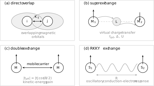
Exchange mechanisms are classified by the electronic process that transmits spin-state dependence. Direct exchange uses overlapping magnetic orbitals; superexchange uses virtual charge transfer through an intermediate ligand; double exchange gains carrier kinetic energy when core moments align; RKKY exchange uses the oscillatory spin response of itinerant electrons. The arrows show common limiting tendencies, not universal sign rules.

These mechanisms are not mutually exclusive labels for materials. A transition-metal oxide can have antiferromagnetic superexchange, ferromagnetic Hund coupling, weaker direct overlap, and longer-range itinerant exchange simultaneously. The effective $J_{ij}$ is the low-energy sum after the active orbitals and charge fluctuations have been specified.

Direct Exchange

Direct exchange couples magnetic orbitals that overlap without requiring a distinct ligand or conduction sea as mediator. At the two-orbital level, its characteristic Coulomb contribution is the exchange integral

$$K_{ij} = \iint d\mathbf r\,d\mathbf r'\, \phi_i^*(\mathbf r) \phi_j(\mathbf r) \frac{e^2}{ 4\pi\epsilon |\mathbf r-\mathbf r'| } \phi_j^*(\mathbf r') \phi_i(\mathbf r').$$

It depends on the transition density $\phi_i^*\phi_j$, so it decreases rapidly as localized orbitals separate. Orbital orientation, radial extent, screening, covalency, and orthogonalization all matter.

For fixed orthonormal orbitals, the bare Coulomb exchange term lowers the triplet relative to the singlet and maps to a ferromagnetic contribution,

$$J_{\mathrm{direct}}^{(V)} = -2K_{ij}.$$

This equation should not be promoted into a universal sign theorem for an interatomic bond. Once orbital relaxation and hopping are allowed, virtual charge fluctuations often add an antiferromagnetic term. What a fitted model calls “nearest-neighbor exchange” may be the sum of both.

Intra-atomic Hund exchange

Different orbitals on the same ion also have direct Coulomb exchange. A common local convention writes

$$H_{\mathrm{Hund}} = - J_{\mathrm H} \sum_{m<m'} \mathbf s_{im}\cdot\mathbf s_{im'}, \qquad J_{\mathrm H}>0.$$

This favors a high-spin atomic multiplet. Hund exchange is crucial in both superexchange and double exchange, but it is not identical to an intersite Heisenberg coupling. Crystal-field splitting, pair hopping, and the full multiorbital Coulomb tensor are needed for quantitative work.

Superexchange

Superexchange is an indirect coupling generated by virtual hopping through high-energy charge configurations. It is especially important in magnetic insulators, where real dc charge transport is suppressed but virtual charge transfer remains allowed.

Two-site Hubbard derivation

The cleanest example is the repulsive two-site Hubbard model,

$$\begin{aligned} H ={}& - t \sum_{\sigma} \left( c_{1\sigma}^{\dagger}c_{2\sigma} + c_{2\sigma}^{\dagger}c_{1\sigma} \right) \\ &+ U \sum_{i=1}^{2} n_{i\uparrow}n_{i\downarrow}, \qquad U>0. \end{aligned}$$

At half filling and $|t|\ll U$, the low-energy subspace has one electron on each site. A hop temporarily creates one empty site and one doubly occupied site, costing energy $U$. A second hop returns to the low-energy sector.

To second order,

$$H_{\mathrm{eff}} = \frac{4|t|^2}{U} \left( \mathbf s_1\cdot\mathbf s_2 - \frac14 \right)$$

within the singly occupied subspace. The constant is chosen so that the triplet energy shift is zero. The singlet is lowered by $4|t|^2/U$, and therefore

$$J_{\mathrm{SE}} = \frac{4|t|^2}{U} >0.$$

This antiferromagnetic sign follows from Pauli blocking and virtual kinetic energy: the singlet can access the relevant doubly occupied intermediate state, whereas the triplet cannot in a one-orbital model.

The result is controlled only when charge excitations remain well separated:

$$\frac{|t|}{U} \ll 1.$$

Near a metal–insulator transition, higher orders, longer-range hopping, ring exchange, and residual charge fluctuations can become important.

Ligand-mediated superexchange

In a transition-metal–ligand–transition-metal path, a metal $d$ electron can virtually enter a ligand $p$ orbital and return through the neighboring metal site. If $t_{pd}$ is a metal–ligand hopping and $\Delta$ a charge-transfer energy, a schematic downfolding gives

$$t_{\mathrm{eff}} \sim \frac{t_{pd}^2}{\Delta},$$

and an antiferromagnetic scale of order

$$J_{\mathrm{AF}} \sim \frac{4t_{pd}^4}{ \Delta^2 U_{\mathrm{eff}} }.$$

This scaling identifies the small parameters, not a complete material formula. Real denominators include metal and ligand Coulomb repulsions, crystal-field levels, Hund couplings, and multiple orbital paths.

Goodenough–Kanamori–Anderson guidance

Orbital symmetry provides useful qualitative rules:

• a nearly $180^\circ$ path between half-filled orbitals that hybridize with the same ligand orbital commonly gives strong antiferromagnetic exchange;
• a near-$90^\circ$ geometry can suppress that shared-orbital path, allowing ligand or metal Hund coupling to favor ferromagnetic exchange;
• half-filled–empty and half-filled–full combinations can have signs different from the half-filled–half-filled case;
• distortions can change both hopping magnitude and the active orbital channel.

These are chemistry-aware limiting rules, not a lookup table based on bond angle alone. The valence, orbital occupancy, local axes, ligand states, and competing paths must all be specified.

Double Exchange

Double exchange couples mixed-valence local moments through the kinetic energy of a mobile carrier. A minimal form contains hopping and a strong ferromagnetic Hund coupling between the carrier spin and a core moment:

$$\begin{aligned} H ={}& - \sum_{\langle i,j\rangle,\sigma} t_{ij} c_{i\sigma}^{\dagger}c_{j\sigma} \\ &- J_{\mathrm H} \sum_i \mathbf S_i\cdot\mathbf s_i, \qquad J_{\mathrm H}>0. \end{aligned}$$

In the strong-$J_{\mathrm H}$ limit, the carrier spin follows the local core-spin direction. If neighboring core moments subtend an angle $\theta_{ij}$, the overlap of their aligned spinors has magnitude

$$\left| \left\langle \chi_i \middle| \chi_j \right\rangle \right| = \cos\frac{\theta_{ij}}{2}.$$

The effective hopping is therefore

$$|t_{ij}^{\mathrm{eff}}| = |t_{ij}| \cos\frac{\theta_{ij}}{2}.$$

Parallel moments maximize the carrier bandwidth and can lower the occupied-band kinetic energy. Antiparallel moments suppress hopping in the ideal limit. This produces a ferromagnetic tendency tied to carrier motion.

Double exchange differs from superexchange in three decisive ways:

Property	Superexchange	Double exchange
Charge process	Virtual excursion and return	Real carrier delocalization
Typical regime	Integer filling, charge localized	Mixed valence or partial filling
Energy scale	Often proportional to $t^2/U$	Often proportional to occupied-band kinetic energy
Angular form	Bilinear at leading order	Can scale as $\cos(\theta/2)$ and be non-Heisenberg

The ferromagnetic tendency is not unconditional. At an empty or completely filled active band there may be no kinetic-energy gain, and antiferromagnetic superexchange between core moments can compete strongly. Lattice distortions, orbital order, polarons, and phase separation can also reshape the simple picture.

RKKY Interaction Preview

The Ruderman–Kittel–Kasuya–Yosida interaction couples localized moments through the spin susceptibility of itinerant carriers. Suppose

$$H_K = J_K \sum_a \mathbf S_a\cdot \mathbf s(\mathbf R_a)$$

couples each local moment to the conduction-electron spin density. To second order in weak $J_K$, integrating out the carriers produces

$$H_{\mathrm{RKKY}} = \sum_{a<b} J_{ab}^{\mathrm{RKKY}} \mathbf S_a\cdot\mathbf S_b,$$

with

$$J_{ab}^{\mathrm{RKKY}} = J_K^2 F(\mathbf R_a-\mathbf R_b).$$

The range function $F$ is a real-space transform of the static spin susceptibility. For a three-dimensional isotropic free-electron gas, its radial dependence can be written, up to an overall convention-dependent positive scale, as

$$F_3(R) \propto \frac{ x\cos x-\sin x }{ x^4 }, \qquad x=2k_{\mathrm F}R.$$

At large distance,

$$F_3(R) \sim \frac{ \cos(2k_{\mathrm F}R+\varphi) }{ R^3 }.$$

The coupling alternates between ferro- and antiferromagnetic sign as distance or carrier density changes. In a crystal, the actual oscillation periods and directions are set by the full Fermi surface rather than one spherical $k_{\mathrm F}$. Dimensionality, disorder, finite temperature, spin–orbit coupling, and multiple bands modify the decay and tensor structure.

RKKY is a weak-coupling result. When the same antiferromagnetic $J_K$ becomes strong, Kondo screening competes with intermoment order. RKKY Interaction owns the sign-complete susceptibility derivation, range function, Fermi-surface geometry, and ordering consequences. Kondo Effect owns the single-impurity screening crossover, while Kondo Lattices owns the Doniach comparison and dense-lattice phases.

Exchange Beyond an Isotropic Scalar

Spin–orbit coupling and low bond symmetry allow a general bilinear tensor,

$$H_{ij} = \mathbf s_i^{\mathsf T} \mathsf J_{ij} \mathbf s_j.$$

Decomposing $\mathsf J_{ij}$ into scalar, antisymmetric, and symmetric-traceless parts gives

$$\begin{aligned} H_{ij} ={}& J_{ij}^{\mathrm{iso}} \mathbf s_i\cdot\mathbf s_j \\ &+ \mathbf D_{ij}\cdot \left( \mathbf s_i\times\mathbf s_j \right) \\ &+ \mathbf s_i\cdot \mathsf\Gamma_{ij} \mathbf s_j. \end{aligned}$$

Here:

• $J_{ij}^{\mathrm{iso}}=\operatorname{Tr}\mathsf J_{ij}/3$ is isotropic exchange;
• $\mathbf D_{ij}$ is the Dzyaloshinskii–Moriya vector;
• $\mathsf\Gamma_{ij}$ is symmetric anisotropic exchange.

An inversion center at the midpoint of a bond forbids $\mathbf D_{ij}$ for that bond. Broken inversion is necessary but not sufficient; the remaining point-group operations constrain its direction. Strong spin–orbit-coupled materials can also generate bond-dependent Ising, compass, or Kitaev-like terms. Spin–Orbit Coupling in Solids explains how local orbital physics and crystal symmetry feed these effective interactions.

Single-ion anisotropy, magnetic dipole interactions, and Zeeman coupling are not exchange, even though they coexist in the same spin Hamiltonian. Magnetic Anisotropy owns their orientation-dependent material consequences and their competition with anisotropic exchange.

What Sets Sign and Strength

An exchange parameter is controlled by several linked scales:

Distance and orbital orientation

Direct overlap and hopping usually decrease rapidly with distance. Because superexchange is proportional to several hopping amplitudes, modest bond-length or bond-angle changes can strongly alter $J$. Pressure, epitaxial strain, and structural transitions can therefore tune exchange.

Occupancy and charge gaps

Virtual exchange denominators depend on onsite repulsion, charge-transfer energy, crystal-field splitting, and Hund coupling. Changing valence or gating a narrow band can move the system between superexchange-dominated and carrier-mediated regimes.

Fermi-surface geometry

RKKY and itinerant exchange inherit wavevectors and anisotropy from the susceptibility $\chi(\mathbf q)$. Nesting, multiple pockets, and spin–orbit splitting can select noncollinear or long-period order.

Competing paths

Two bonds of equal length need not have equal exchange if their ligand chemistry differs. Several paths can cancel, making a small net $J$ highly sensitive to structural details. A sign change is often evidence for competition, not for one mechanism changing its intrinsic nature.

Choice of low-energy model

Downfolding into different orbital sets redistributes physics among hopping, onsite interactions, and exchange terms. A static pairwise $J_{ij}$ extracted near one reference state can differ from a coupling fitted over large spin rotations or at another temperature. Exchange parameters are model coordinates, not basis-independent observables.

How Exchange Is Determined

No single measurement reads out every $J_{ij}$ directly. Reliable inference combines complementary information.

Singlet–triplet spectroscopy

For an isolated spin-$1/2$ dimer in this convention,

$$J = E_T-E_S.$$

Inelastic neutron scattering, electron-spin resonance, optical spectroscopy, or tunneling spectroscopy can resolve this gap. Extra anisotropy splits the triplet and must be included rather than absorbed blindly into one $J$.

Magnon dispersion

In an ordered magnet, exchange controls the momentum dependence of spin-wave energies. Inelastic neutron scattering measures the dynamic structure factor $S(\mathbf q,\omega)$, allowing multiple neighbor couplings to be fitted across the Brillouin zone. Magnons owns the quantization and spectral-weight framework.

A zone-center stiffness alone usually constrains only a weighted moment of the $J_{ij}$. Several exchange networks can share the same long-wavelength slope but differ at the zone boundary.

Thermodynamics

Susceptibility, specific heat, and ordering temperature constrain exchange scales, but they are inverse problems. Frustration, dimensionality, anisotropy, disorder, and quantum fluctuations can suppress the ordering temperature far below the largest bond energy. The estimate $k_{\mathrm B}T_{\mathrm{ord}}\sim J$ is dimensional guidance, not an extraction formula.

Electronic-structure mapping

One can calculate total energies for several magnetic configurations and fit them to a spin Hamiltonian. For one isolated classical pair of equal spin length $s$,

$$E_{\parallel} -E_{\mathrm{antiparallel}} = 2Js^2.$$

In a lattice, bond multiplicities and all simultaneously changed pairs must be counted. The fitted result depends on the spin normalization, reference state, electronic-structure approximation, orbital projection, and chosen interaction terms.

Infinitesimal-rotation or magnetic-force-theorem methods extract the curvature of electronic energy around a reference state. Correlated methods can add frequency-dependent self-energies and vertex information. Agreement with measured magnon dispersions is a stronger test than agreement with one collinear energy difference.

When a Heisenberg Mapping Is Valid

A static pairwise spin model is most credible when:

• robust local moments persist over the energy and temperature range of interest;
• charge and orbital excitations are separated from spin dynamics;
• spin rotations are slow compared with electronic adjustment;
• the energy is approximately bilinear over the relevant angular range;
• generated multispin and anisotropic terms are small or explicitly retained.

The mapping can fail or need extension when:

• moment magnitude changes substantially during a rotation;
• the magnetism is itinerant and inseparable from Fermi-surface reconstruction;
• charge fluctuations are not perturbative;
• orbital degeneracy produces coupled spin–orbital dynamics;
• ring exchange, biquadratic exchange, or multipolar interactions are comparable to $J$;
• the effective interaction is retarded or strongly temperature dependent;
• disorder creates a broad distribution of bond strengths.

The correct response is not to abandon effective models, but to enlarge the retained degrees of freedom and report the regime in which the parameters were obtained.

Mechanism Comparison

Mechanism	Electronic path	Common range	Characteristic control	Typical warning
Direct exchange	Overlap of magnetic orbitals	Short	Transition density and Coulomb integral	Bare triplet preference is not the full bond energy
Superexchange	Virtual hopping through charge states or ligand	Usually short to intermediate	$t^2/U$ or charge-transfer denominators	Bond angle alone does not fix the sign
Double exchange	Real carrier hopping between Hund-aligned sites	Band-scale	Filling, bandwidth, and $J_{\mathrm H}$	Angular energy can be non-Heisenberg
RKKY	Itinerant spin susceptibility	Long and oscillatory	Fermi surface and $J_K^2$	Weak-coupling and clean-host assumptions matter
Anisotropic exchange	Spin–orbit-coupled virtual processes	Bond dependent	Point-group symmetry and spin–orbit scale	Scalar $J$ cannot encode chirality

Reliable Interpretation Workflow

1. Declare the Hamiltonian convention. Fix sign, spin normalization, bond counting, and units.
2. Identify retained degrees of freedom. State which orbitals, local multiplets, carriers, and ligands remain explicit.
3. Name the virtual or itinerant process. Draw the intermediate states and their energy denominators.
4. Check the small parameter. Examples include $t/U$, $t_{pd}/\Delta$, or weak $J_K$.
5. Use symmetry before fitting. Determine which isotropic, Dzyaloshinskii–Moriya, and symmetric-anisotropic terms are allowed.
6. Fit more than one observable. Combine energies, dispersion, intensity, susceptibility, and structural trends.
7. Test transferability. Vary reference state, fitting window, temperature, pressure, or orbital basis.
8. Report uncertainty and omitted terms. A list of $J_{ij}$ without its model contract is incomplete.

Common mistakes

• Calling exchange a separate classical force or a literal particle-exchange event.
• Saying Pauli exclusion always favors ferromagnetism.
• Forgetting that $J>0$ and $J<0$ reverse meaning under another Hamiltonian convention.
• Treating every insulating magnetic bond as antiferromagnetic superexchange.
• Using bond angle without orbital occupancy and local symmetry.
• Calling double exchange a second-order $t^2/U$ process.
• Inferring a unique RKKY period from one spherical carrier density in a multiband crystal.
• Equating a density-functional exchange-correlation functional with an intersite $J_{ij}$.
• Estimating $J$ directly from an ordering temperature while ignoring dimensionality and frustration.
• Treating exchange parameters extracted near one state as immutable material constants.

Exercises

1. Dimer sign audit

For

$$H = J\mathbf s_1\cdot\mathbf s_2$$

with two spin-$1/2$ moments, derive the singlet and triplet energies. Which state is lower for each sign of $J$?

Solution

Using

$$\mathbf s_1\cdot\mathbf s_2 = \frac12 \left[ s_{\mathrm{tot}}(s_{\mathrm{tot}}+1) - \frac34 - \frac34 \right],$$

the singlet has $s_{\mathrm{tot}}=0$ and the triplet has $s_{\mathrm{tot}}=1$. Therefore

$$E_S = -\frac{3J}{4}, \qquad E_T = \frac{J}{4}.$$

For $J>0$, the singlet is lower and the coupling is antiferromagnetic. For $J<0$, the triplet is lower and the coupling is ferromagnetic.

2. Direct exchange and spatial separation

Show that the Coulomb contribution from two fixed orthonormal orbitals gives $E_T-E_S=-2K_{ab}$. What happens when the orbitals have disjoint support?

Solution

The spatial singlet partner is symmetric and has interaction energy $C_{ab}+K_{ab}$. The triplet partner is antisymmetric and has energy $C_{ab}-K_{ab}$. Hence

$$E_T-E_S = \left(C_{ab}-K_{ab}\right) - \left(C_{ab}+K_{ab}\right) = -2K_{ab}.$$

If the orbitals have disjoint support, the transition density $a^*(\mathbf r)b(\mathbf r)$ vanishes, so $K_{ab}=0$. Exchange antisymmetry remains exact, but this interaction no longer splits the spin states.

3. Hubbard superexchange

In the half-filled two-site Hubbard model with $U\gg|t|$, the triplet has no second-order energy shift while the singlet shifts by $-4|t|^2/U$. Determine the effective Heisenberg coupling and constant term.

Solution

Write

$$H_{\mathrm{eff}} = A + J\mathbf s_1\cdot\mathbf s_2.$$

The triplet and singlet energies are

$$A+\frac{J}{4} = 0, \qquad A-\frac{3J}{4} = -\frac{4|t|^2}{U}.$$

Subtracting gives

$$J = \frac{4|t|^2}{U},$$

and then $A=-J/4=-|t|^2/U$. Thus

$$H_{\mathrm{eff}} = \frac{4|t|^2}{U} \left( \mathbf s_1\cdot\mathbf s_2-\frac14 \right).$$

4. Spinor overlap in double exchange

Let

$$|\chi(\theta,\phi)\rangle = \begin{pmatrix} \cos(\theta/2)\\ e^{i\phi}\sin(\theta/2) \end{pmatrix}$$

represent a spin aligned with a unit vector. Show that the magnitude of the overlap of two aligned spinors separated by angle $\Theta$ is $\cos(\Theta/2)$.

Solution

For pure spin-$1/2$ states with Bloch vectors $\mathbf n_i$ and $\mathbf n_j$,

$$\left| \langle\chi_i|\chi_j\rangle \right|^2 = \frac{ 1+\mathbf n_i\cdot\mathbf n_j }{2}.$$

Since $\mathbf n_i\cdot\mathbf n_j=\cos\Theta$,

$$\left| \langle\chi_i|\chi_j\rangle \right|^2 = \frac{1+\cos\Theta}{2} = \cos^2\frac{\Theta}{2}.$$

For $0\le\Theta\le\pi$, the magnitude is $\cos(\Theta/2)$. Parallel core spins maximize hopping; antiparallel spins suppress it in the ideal strong-Hund limit.

5. RKKY oscillation scale

Using the asymptotic form

$$J(R) \propto \frac{\cos(2k_{\mathrm F}R+\varphi)}{R^3},$$

find the spatial period of the oscillation and the spacing between successive sign changes.

Solution

Increasing $R$ by $\Delta R$ changes the cosine phase by $2k_{\mathrm F}\Delta R$. A full period requires

$$2k_{\mathrm F}\Delta R = 2\pi,$$

so

$$\Delta R_{\mathrm{period}} = \frac{\pi}{k_{\mathrm F}}.$$

Successive zero crossings are separated by half that distance:

$$\Delta R_{\mathrm{zero}} = \frac{\pi}{2k_{\mathrm F}}.$$

In a crystal, several Fermi-surface spanning vectors can produce several oscillation scales.

6. Why midpoint inversion forbids Dzyaloshinskii–Moriya exchange

Consider

$$H_{\mathrm{DM}} = \mathbf D_{ij}\cdot \left( \mathbf s_i\times\mathbf s_j \right).$$

Show why an inversion center at the bond midpoint requires $\mathbf D_{ij}=0$.

Solution

Inversion about the midpoint exchanges sites $i$ and $j$. Spin is an axial vector, so each spin direction is unchanged by spatial inversion, but the site labels swap:

$$\mathbf s_i\times\mathbf s_j \longrightarrow \mathbf s_j\times\mathbf s_i = - \mathbf s_i\times\mathbf s_j.$$

The bond is mapped onto itself. Invariance would therefore require the same coefficient multiplying both a term and its negative. The only possibility is $\mathbf D_{ij}=0$.

7. Energy-mapping normalization

A calculation uses two classical spins of length $s=3/2$ and the convention $H=J\mathbf s_1\cdot\mathbf s_2$. It finds $E_{\parallel}-E_{\mathrm{antiparallel}}=-18\,\mathrm{meV}$ for an isolated pair. Determine $J$ and its magnetic sign.

Solution

For parallel and antiparallel classical vectors,

$$E_{\parallel} = Js^2, \qquad E_{\mathrm{antiparallel}} = -Js^2.$$

Thus

$$2Js^2 = -18\,\mathrm{meV}.$$

With $s^2=9/4$,

$$J = \frac{-18\,\mathrm{meV}}{2(9/4)} = -4\,\mathrm{meV}.$$

The negative sign is ferromagnetic in this convention. In a lattice calculation, every changed bond and any moment-length change would also need to be counted.

Connections

• Magnetic Moments in Matter tests whether a stable moment or projected pseudospin manifold exists and fixes its normalization before this page assigns microscopic exchange couplings.
• Silicon Spin Qubits uses tunable two-spin exchange as a gate primitive and tracks pulse area, charge-noise sensitivity, leakage, routing, and code-cycle consequences.
• Spin and Spatial Wavefunctions owns the fermionic symmetry bookkeeping behind singlet and triplet spatial states.
• Exchange and Correlation develops direct and exchange integrals, exchange holes, and mean-field accounting.
• Hubbard Model owns the lattice model whose strong-coupling limit generates $J=4t^2/U$.
• t–J Model follows exchange into a projected, doped material model and audits charge-transfer and cuprate reductions.
• Schrieffer–Wolff Transformation gives the controlled block-diagonalization used to eliminate virtual charge states.
• Heisenberg Model owns exact dimer, chain, symmetry, frustration, and dimensionality results for the isotropic spin model.
• Kondo Model Preview introduces the local exchange whose weak-coupling square produces RKKY interactions.
• RKKY Interaction derives susceptibility-mediated exchange, the Lindhard range function, Fermi-surface directionality, and ordering wavevectors.
• Kondo Effect develops material screening, resistance minima, operational Kondo scales, and the competition with intermoment order.
• Fermi Surface supplies the itinerant geometry governing long-range susceptibility oscillations.
• Ferromagnetism shows how exchange can support uniform magnetic order while domains, anisotropy, and itinerancy determine material behavior.
• Antiferromagnetism follows antiferromagnetic couplings into Néel order, competing wavevectors, spin flop, frustration, and localized or itinerant material regimes.
• Ferrimagnetism shows how antiferromagnetic intersublattice coupling plus unequal moments yields uncompensated order and acoustic and optical collective modes.
• Skyrmions and Magnetic Textures develops how exchange, frustration, and Dzyaloshinskii–Moriya coupling enter domain walls, vortices, and topological spin textures.
• Magnons explains how exchange becomes a measured spin-wave dispersion and spectral response.
• Spin Waves and Magnons in Materials develops the forward model from an exchange network and ordered structure to energies, eigenvectors, probe intensities, and fitted parameters.
• Condensed-Matter Roadmap places exchange between local quantum states, electronic structure, and collective magnetism.

References

1. P. A. M. Dirac, “On the Theory of Quantum Mechanics,” Proceedings of the Royal Society A 112, 661–677 (1926), doi:10.1098/rspa.1926.0133.
2. W. Heisenberg, “Zur Theorie des Ferromagnetismus,” Zeitschrift für Physik 49, 619–636 (1928), doi:10.1007/BF01328601.
3. P. W. Anderson, “Antiferromagnetism. Theory of Superexchange Interaction,” Physical Review 79, 350–356 (1950), doi:10.1103/PhysRev.79.350.
4. P. W. Anderson, “New Approach to the Theory of Superexchange Interactions,” Physical Review 115, 2–13 (1959), doi:10.1103/PhysRev.115.2.
5. J. B. Goodenough, “Theory of the Role of Covalence in the Perovskite-Type Manganites,” Physical Review 100, 564–573 (1955), doi:10.1103/PhysRev.100.564.
6. J. Kanamori, “Superexchange interaction and symmetry properties of electron orbitals,” Journal of Physics and Chemistry of Solids 10, 87–98 (1959), doi:10.1016/0022-3697(59)90061-7.
7. C. Zener, “Interaction between the d-Shells in the Transition Metals. II. Ferromagnetic Compounds of Manganese with Perovskite Structure,” Physical Review 82, 403–405 (1951), doi:10.1103/PhysRev.82.403.
8. P. W. Anderson and H. Hasegawa, “Considerations on Double Exchange,” Physical Review 100, 675–681 (1955), doi:10.1103/PhysRev.100.675.
9. M. A. Ruderman and C. Kittel, “Indirect Exchange Coupling of Nuclear Magnetic Moments by Conduction Electrons,” Physical Review 96, 99–102 (1954), doi:10.1103/PhysRev.96.99.
10. T. Kasuya, “A Theory of Metallic Ferro- and Antiferromagnetism on Zener’s Model,” Progress of Theoretical Physics 16, 45–57 (1956), doi:10.1143/PTP.16.45.
11. K. Yosida, “Magnetic Properties of Cu-Mn Alloys,” Physical Review 106, 893–898 (1957), doi:10.1103/PhysRev.106.893.
12. T. Moriya, “Anisotropic Superexchange Interaction and Weak Ferromagnetism,” Physical Review 120, 91–98 (1960), doi:10.1103/PhysRev.120.91.
13. A. Szilva, Y. Kvashnin, E. A. Stepanov, L. Nordström, O. Eriksson, A. I. Lichtenstein, and M. I. Katsnelson, “Quantitative theory of magnetic interactions in solids,” Reviews of Modern Physics 95, 035004 (2023), doi:10.1103/RevModPhys.95.035004.
14. D. I. Khomskii, Transition Metal Compounds (Cambridge University Press, 2014), doi:10.1017/CBO9781139096782.