Spintronics

Spintronics studies how spin angular momentum and magnetic order are generated, transported, detected, and used to control electronic or magnetic states. Its central objects are not isolated spins but nonequilibrium spin accumulations, spin-polarized charge currents, pure spin currents, interfacial torques, and magnetization-dependent electrical signals.

A useful device separates four functions:

1. generation, by a ferromagnetic contact, optical orientation, the spin Hall effect, or interfacial spin–momentum locking;
2. transport, by itinerant electrons, holes, magnons, or collective magnetic order;
3. manipulation, by precession, exchange fields, spin–orbit fields, spin-transfer torque, or spin–orbit torque;
4. detection, through a ferromagnetic analyzer, inverse charge–spin conversion, magnetoresistance, optical rotation, or magnetic resonance.

Those stages are linked by interfaces. A large bulk polarization or spin Hall conductivity does not guarantee a large device signal if the interface absorbs, depolarizes, reflects, or shunts the relevant current.

Density and Current Operators owns microscopic current operators and the nonuniqueness of spin current when spin is not conserved. Spin–Orbit Coupling in Solids owns intrinsic and extrinsic spin Hall mechanisms. This page owns the device-level transport ledger: spin diffusion and injection, nonlocal detection, giant magnetoresistance, reciprocal conversion, spin pumping, current-induced torques, and the material constraints connecting them.

Required background. Density and Current Operators supplies spin-current and torque definitions, while Spin–Orbit Coupling in Solids supplies charge–spin conversion mechanisms.

Helpful background. Ferromagnetism provides injection and magnetoresistive context, while Boltzmann Transport provides the semiclassical transport closure.

Convention and unit ledger

Spin-transport literature uses several quantities all called “spin current.” They are not numerically interchangeable.

Let $e>0$ denote the elementary charge. A spin-resolved conventional charge-current density has units $\mathrm{A\,m^{-2}}$. For a chosen quantization axis,

$$\mathbf j_c = \mathbf j_\uparrow + \mathbf j_\downarrow , \qquad \mathbf j_s^{(q)} = \mathbf j_\uparrow - \mathbf j_\downarrow .$$

The superscript $(q)$ marks the charge-equivalent normalization. Its current polarization is

$$P_j = \frac{ \mathbf j_s^{(q)}\cdot\hat{\mathbf n} }{ \mathbf j_c\cdot\hat{\mathbf n} } = \frac{ j_\uparrow-j_\downarrow }{ j_\uparrow+j_\downarrow },$$

for transport along $\hat{\mathbf n}$. This scalar description is adequate only when a common spin axis remains meaningful.

The angular-momentum-current tensor $Q_i^{\,a}$ describes flow along spatial direction $i$ of spin angular momentum polarized along $a$. Its units are angular momentum per area per time. We define

$$j_{s,i}^{\,a} \equiv \frac{2e}{\hbar} Q_i^{\,a},$$

so $j_{s,i}^{\,a}$ also has units $\mathrm{A\,m^{-2}}$. The inverse relation is

$$Q_i^{\,a} = \frac{\hbar}{2e} j_{s,i}^{\,a}.$$

Some authors call $Q_i^{\,a}$ the spin current; others call $j_{s,i}^{\,a}$ the spin current and suppress the factor $\hbar/2e$. Every quoted spin Hall angle, interface conductance, or torque efficiency should therefore state its normalization.

For collinear transport, the spin accumulation is the splitting of spin-resolved electrochemical potentials,

$$\mu_s \equiv \mu_\uparrow-\mu_\downarrow .$$

For noncollinear transport it becomes a vector $\boldsymbol{\mu}_s$ in spin space. It has units of energy, not magnetization. A spin density and a spin accumulation are related through the appropriate density of states and susceptibility; they are not identical variables.

We use:

• $\mathbf m=\mathbf M/M_s$ for a ferromagnet’s unit magnetization;
• $\hat{\mathbf p}$ for the injected spin-polarization direction;
• $t_F$ for the active magnetic-layer thickness;
• $\lambda_s$ for a spin-diffusion length;
• $\tau_s$ for a spin-relaxation time;
• $\theta_{\mathrm{SH}}$ for a spin Hall conversion ratio in an explicitly stated geometry;
• $g_{\mathrm{eff}}^{\uparrow\downarrow}$ for an effective spin-mixing conductance per area.

Current direction, electron-flow direction, interface normal, and magnetization direction must be drawn separately. Reversing any one of them can reverse a reported sign.

Spin continuity and diffusion

For spin density $s^a$, a local balance equation has the form

$$\frac{\partial s^a}{\partial t} + \partial_i Q_i^{\,a} = \mathcal T^a - \frac{s^a-s_{\mathrm{eq}}^a}{\tau_{\mathrm{sf}}},$$

where $\mathcal T^a$ is a coherent torque density and the final term represents a simple spin-flip relaxation model. When the Hamiltonian does not conserve $s^a$, current and torque can be repartitioned by torque-dipole terms. The measurable content lies in the complete balance law and boundary conditions, not in a current symbol alone.

In a diffusive nonmagnetic conductor, a widely used phenomenological equation is

$$\frac{\partial\boldsymbol{\mu}_s}{\partial t} = D_s\nabla^2\boldsymbol{\mu}_s - \frac{\boldsymbol{\mu}_s}{\tau_s} + \boldsymbol{\Omega}_L \times \boldsymbol{\mu}_s + \mathbf S,$$

where $D_s$ is a spin-diffusion coefficient, $\boldsymbol{\Omega}_L$ is the Larmor-frequency vector, and $\mathbf S$ is a source. Without precession or a source, each steady component obeys

$$\nabla^2\mu_s = \frac{\mu_s}{\lambda_s^2}, \qquad \lambda_s = \sqrt{D_s\tau_s}.$$

In one dimension,

$$\mu_s(x) = A e^{-x/\lambda_s} + B e^{x/\lambda_s}.$$

Boundary conditions discard the exponentially growing branch in a semi-infinite lead. The diffusion length is therefore not the mean free path: it combines many momentum-scattering events with a slower loss of spin memory.

If $\zeta_\sigma$ is a spin-resolved electrochemical potential expressed in volts, define

$$\zeta_s = \zeta_\uparrow-\zeta_\downarrow .$$

For equal spin-channel conductivities in a nonmagnetic metal,

$$\mathbf j_s^{(q)} = - \frac{\sigma}{2} \boldsymbol{\nabla}\zeta_s .$$

The sign follows this voltage convention. If $\mu_s$ is used instead, the conversion between $\mu_s$ and $\zeta_s$ must be stated. This small bookkeeping choice explains many apparent sign disagreements.

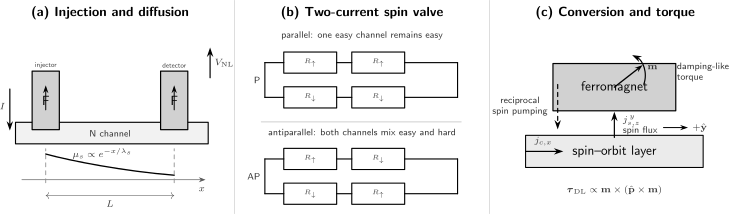
Three device ledgers. (a) A ferromagnetic injector creates a spin accumulation that decays over $\lambda_s$ in a nonmagnetic channel and is sampled nonlocally by a second ferromagnet. (b) A two-current resistor model gives low resistance for parallel magnetic layers and high resistance for antiparallel layers. (c) A charge current in a spin–orbit layer generates a transverse spin flux into a ferromagnet, producing a damping-like torque; reciprocal spin pumping emits angular momentum from a precessing magnet.

Spin injection across an interface

Consider a ferromagnet F, a nonmagnetic channel N, and an interface c. In a one-dimensional collinear diffusion model it is useful to compare spin-resistance-area products,

$$r_N = \rho_N\lambda_N,$$

and

$$r_F = \frac{ \rho_F\lambda_F }{ 1-P_F^2 }.$$

Here $P_F$ is the bulk conductivity polarization. Both $r_N$ and $r_F$ have units $\Omega\,\mathrm{m^2}$. Let $r_c$ and $P_c$ denote the contact’s spin-averaged resistance-area product and polarization in a specified interface convention. A common idealized injection result is

$$P_{\mathrm{inj}} \simeq \frac{ P_F r_F + P_c r_c }{ r_F+r_N+r_c }.$$

Exact factors depend on whether spin-channel resistances, total contact resistance, or area-normalized conductances are used. The physical limits are more robust than any memorized prefactor:

$$\begin{aligned} r_N\gg r_F,r_c &\Longrightarrow P_{\mathrm{inj}}\ll P_F, \\ r_c\gg r_F,r_N &\Longrightarrow P_{\mathrm{inj}}\to P_c. \end{aligned}$$

The first limit is the conductivity-mismatch problem for a transparent ferromagnet–semiconductor contact: the channel’s large spin resistance suppresses injection. A spin-selective tunnel barrier can raise $r_c$ and restore polarization. An arbitrarily resistive barrier is not automatically optimal, because it reduces charge current, signal bandwidth, and impedance matching.

Real interfaces add:

• spin-dependent interface transmission;
• spin-memory loss from interfacial disorder and spin–orbit coupling;
• interface states and Fermi-level pinning;
• current crowding and nonuniform contact geometry;
• magnon-assisted and inelastic channels;
• proximity magnetism and intermixing.

Bulk polarization, contact polarization, and the polarization delivered to the channel are therefore distinct experimental quantities.

Nonlocal detection and Hanle precession

In a lateral nonlocal geometry, one ferromagnet injects current into a nonmagnetic channel while a distant ferromagnet detects voltage in a nominally open circuit. This separation strongly suppresses ordinary charge-voltage backgrounds.

For a narrow one-dimensional channel, an ideal form is

$$R_{\mathrm{NL}} \equiv \frac{V_{\mathrm{NL}}}{I} \simeq \pm P_{\mathrm{inj}}P_{\mathrm{det}} R_N e^{-L/\lambda_N},$$

where

$$R_N = \frac{\rho_N\lambda_N}{A_N}.$$

The sign changes between parallel and antiparallel injector–detector magnetizations. Some papers define $\Delta R_{\mathrm{NL}}$ as the full parallel-minus-antiparallel difference, which adds a factor of two. Finite contact widths, spin absorption, multidimensional spreading, and interface resistances change the prefactor.

A transverse field rotates the diffusing spins. For injection along one spin axis, the ideal Hanle response contains

$$\begin{aligned} R_{\mathrm{NL}}(B) \propto \int_0^\infty & \frac{\mathrm dt}{ \sqrt{4\pi D_s t} } \exp \left( - \frac{L^2}{4D_s t} - \frac{t}{\tau_s} \right) \\ &\times \cos(\Omega_L t). \end{aligned}$$

The diffusion kernel sums over all travel times; the cosine records precession. The characteristic dephasing field satisfies roughly

$$|\Omega_L|\tau_s \sim 1, \qquad \boldsymbol{\Omega}_L = \frac{g\mu_B}{\hbar}\mathbf B$$

for an isotropic $g$ factor. Reliable extraction of $D_s$ and $\tau_s$ may require contact-induced relaxation, drift, anisotropic $g$ tensors, stray fields, nuclear fields, and magnetic switching to be modeled rather than absorbed into a single Lorentzian.

Giant magnetoresistance

Giant magnetoresistance (GMR) is the dependence of a metallic multilayer’s resistance on the relative orientation of neighboring magnetic layers. It is a nonequilibrium transport effect, not simply the equilibrium energy that favors one alignment.

The Mott two-current picture begins with weak spin-flip scattering: majority and minority carriers conduct approximately in parallel and experience different resistances. For two identical ferromagnetic layers, let $R_\uparrow$ and $R_\downarrow$ be the resistance of one layer for spin quantized along its magnetization. In the parallel state,

$$R_P = \frac{ 2R_\uparrow R_\downarrow }{ R_\uparrow+R_\downarrow }.$$

In the antiparallel state, each channel encounters one majority-like and one minority-like layer, so

$$R_{\mathrm{AP}} = \frac{ R_\uparrow+R_\downarrow }{ 2 }.$$

Thus

$$\frac{ R_{\mathrm{AP}}-R_P }{ R_P } = \frac{ (R_\uparrow-R_\downarrow)^2 }{ 4R_\uparrow R_\downarrow } \ge 0.$$

Defining

$$\beta = \frac{ R_\downarrow-R_\uparrow }{ R_\downarrow+R_\uparrow },$$

the same result becomes

$$\frac{\Delta R}{R_P} = \frac{\beta^2}{1-\beta^2}.$$

This resistor network captures the sign and intuition, but not quantitative multilayers. Current-in-plane (CIP) and current-perpendicular-to-plane (CPP) geometries sample bulk and interface scattering differently. In CPP structures, the Valet–Fert theory solves spin-dependent diffusion with bulk asymmetries, interface resistances, finite spin-diffusion lengths, and spin accumulation. Layer thicknesses much larger than $\lambda_s$ do not contribute coherently to spin contrast throughout their full volume.

Do not merge distinct magnetoresistances

Effect	State variable controlling resistance	Typical structure
Anisotropic magnetoresistance (AMR)	angle between current and one magnetic order parameter	single magnetic conductor
GMR	relative orientation of metallic magnetic layers	metallic spin valve or multilayer
Tunneling magnetoresistance (TMR)	relative orientation across a tunnel barrier	magnetic tunnel junction
Spin Hall magnetoresistance	spin reflection and absorption at a spin–orbit-metal/magnet interface	bilayer
Colossal magnetoresistance (CMR)	coupled magnetic, electronic, and structural state	correlated magnetic oxide

For an ideal spin-conserving tunnel junction, Jullière’s model gives

$$\mathrm{TMR} \equiv \frac{ R_{\mathrm{AP}}-R_P }{ R_P } \simeq \frac{ 2P_1P_2 }{ 1-P_1P_2 },$$

where $P_1$ and $P_2$ are tunneling density-of-states polarizations. Crystalline symmetry filtering, barrier defects, bias, temperature, magnons, and interface resonances can invalidate this simple density-of-states formula.

Charge–spin conversion

Spin–orbit coupling permits reciprocal conversion between longitudinal charge flow and transverse spin flow. To make signs explicit, suppose a charge current flows along $+\hat{\mathbf x}$, spin angular momentum flows along $+\hat{\mathbf z}$, and its polarization is $+\hat{\mathbf y}$. We define the sign of the spin Hall angle by

$$j_{s,z}^{\,y} = \theta_{\mathrm{SH}} j_{c,x}.$$

Changing the interface normal or choosing electron flow instead of conventional current changes the verbal handedness. The tensor relation, axes, and sign convention should accompany every number.

The intrinsic Berry-curvature contribution, skew scattering, side jump, and the conventional spin-current operator are developed in Spin–Orbit Coupling in Solids. At the device level, a measured conversion also depends on

$$t, \quad \lambda_s, \quad \rho, \quad g_{\mathrm{eff}}^{\uparrow\downarrow}, \quad \text{interface transparency}, \quad \text{current shunting}.$$

A fitted torque efficiency is therefore not automatically the intrinsic bulk spin Hall angle.

The inverse spin Hall effect converts an injected spin flux into a transverse charge signal. Onsager reciprocity constrains direct and inverse linear-response coefficients after all time-reversal-odd variables, especially magnetization, are transformed consistently. It does not excuse ignoring open-circuit boundary conditions or sign conventions.

At a two-dimensional inversion-asymmetric interface, the Edelstein effect produces a nonequilibrium spin accumulation from an in-plane electric field. Its reciprocal converts an injected spin accumulation or flux into a two-dimensional charge current. This interfacial spin density is not the same object as a bulk transverse spin Hall current, even though both can generate similar torques.

Spin pumping and interfacial mixing

A precessing magnet can emit spin angular momentum into an adjacent conductor. For a slowly varying unit magnetization, the pumped angular-momentum current per area is

$$\mathbf Q_s^{\mathrm{pump}} = \frac{\hbar}{4\pi} \left[ g_r^{\uparrow\downarrow} \mathbf m\times\dot{\mathbf m} - g_i^{\uparrow\downarrow} \dot{\mathbf m} \right].$$

Here $g_r^{\uparrow\downarrow}$ and $g_i^{\uparrow\downarrow}$ are the real and imaginary parts of the spin-mixing conductance per area in the stated convention. The receiving material develops a backflow spin accumulation; replacing the bare conductance by $g_{\mathrm{eff}}^{\uparrow\downarrow}$ folds that backflow and spin loss into an effective interface parameter.

Spin pumping adds damping to a magnetic film:

$$\Delta\alpha = \frac{ |\gamma|\hbar }{ 4\pi M_s t_F } g_{\mathrm{eff}}^{\uparrow\downarrow}.$$

Inverse spin Hall voltage, terahertz emission, or a nonlocal detector can register the emitted spin current. A linewidth increase alone is not unique proof of spin pumping: two-magnon scattering, radiative damping, eddy currents, inhomogeneous broadening, and magnetic proximity effects require controls.

Spin pumping and spin-transfer torque are reciprocal interfacial processes. One exports angular momentum from a moving magnet; the other absorbs angular momentum from an incident nonequilibrium spin distribution.

Spin-transfer and spin–orbit torques

The Landau–Lifshitz–Gilbert equation with current-induced torques can be written

$$\dot{\mathbf m} = - |\gamma|\mu_0 \mathbf m\times\mathbf H_{\mathrm{eff}} + \alpha \mathbf m\times\dot{\mathbf m} + \boldsymbol{\tau}_{\mathrm{STT}} + \boldsymbol{\tau}_{\mathrm{SOT}}.$$

For a spin flux polarized along $\hat{\mathbf p}$ and absorbed by a uniform magnetic layer, the leading angular structures are

$$\boldsymbol{\tau}_{\mathrm{DL}} = \tau_{\mathrm{DL}} \mathbf m\times \left( \hat{\mathbf p}\times\mathbf m \right),$$

and

$$\boldsymbol{\tau}_{\mathrm{FL}} = \tau_{\mathrm{FL}} \mathbf m\times\hat{\mathbf p}.$$

The first is called damping-like because its symmetry can oppose or reinforce Gilbert damping for a suitable trajectory. The second has the symmetry of precession about an effective field. The names describe vector form, not a unique microscopic origin.

For charge-equivalent injected spin current, a common damping-like coefficient is

$$\tau_{\mathrm{DL}} = \frac{ |\gamma|\hbar }{ 2eM_s t_F } \xi_{\mathrm{DL}}j_c,$$

where $\xi_{\mathrm{DL}}$ includes conversion and transmission. For a spin valve, $\hat{\mathbf p}$ is set by a polarizing magnetic layer and the torque is usually called spin-transfer torque. In a spin–orbit bilayer, $\hat{\mathbf p}$ can be generated by the spin Hall or Edelstein effect and the torque is usually called spin–orbit torque.

In a smoothly varying magnetic texture, current within the magnet also produces adiabatic and nonadiabatic torques:

$$\boldsymbol{\tau}_{\mathrm{texture}} = - (\mathbf u\cdot\boldsymbol{\nabla})\mathbf m + \beta_{\mathrm{na}} \mathbf m\times \left[ (\mathbf u\cdot\boldsymbol{\nabla})\mathbf m \right].$$

The drift parameter $\mathbf u$ is proportional to current polarization, and $\beta_{\mathrm{na}}$ is a nonadiabatic coefficient. This continuum form assumes a texture smooth on microscopic transport scales.

A macrospin switching estimate follows by balancing antidamping torque against magnetic damping:

$$j_c^{\mathrm{crit}} \sim \frac{ 2e }{ \hbar } \frac{ \alpha M_s t_F }{ \xi_{\mathrm{DL}} } \mu_0H_{\mathrm{eff}}.$$

Its coefficient depends on geometry, demagnetizing fields, pulse duration, temperature, incubation, and the angular dependence of torque. Real switching often proceeds by domain nucleation and wall motion rather than coherent rotation. A quoted critical current without pulse width and error probability is incomplete.

Materials and devices

No single figure of merit ranks all spintronic materials. A useful ledger includes:

Platform	Main function	Useful attributes	Frequent limitation
Metallic ferromagnet/nonmagnet	injection, GMR, spin torque	high current density, mature interfaces	short $\lambda_s$, Joule heating
Magnetic tunnel junction	TMR readout, STT switching	large resistance contrast, nonvolatility	barrier defects, write stress, stochastic switching
Heavy spin–orbit metal or semimetal	spin Hall generation and inverse detection	efficient charge–spin conversion	shunting, resistive loss, interface uncertainty
Semiconductor or two-dimensional channel	gate control, long-distance transport	tunable density and spin–orbit coupling	contact mismatch, disorder, environmental sensitivity
Magnetic insulator	magnon transport, spin pumping	negligible electronic charge current in magnet	interface conversion and magnon relaxation
Antiferromagnet or ferrimagnet	fast dynamics, compensated or low-moment operation	weak stray fields, rich torque symmetry	readout, domain control, material variability

Read and write architectures

Metallic spin valves and GMR multilayers enabled compact magnetic-field sensors and hard-disk read heads. A magnetic tunnel junction uses TMR to distinguish a free layer from a reference layer. In spin-transfer-torque MRAM, the current used to read the tunnel junction also passes through it during writing. In many spin–orbit-torque designs, a lateral current in an adjacent layer writes a magnetic element while the tunnel junction provides a separate read path.

The magnetic energy barrier must satisfy

$$\Delta \equiv \frac{E_b}{k_BT}$$

large enough for retention, while write torque must still cross the barrier quickly and reliably. Magnetic Anisotropy owns the barrier, anisotropy, and thermal-activation ledger. Lowering $E_b$ reduces write cost but also retention; increasing damping can accelerate settling while raising antidamping current.

Other platforms extend the same generation–transport–manipulation–detection logic:

• semiconductor spin transistors seek electrical control of precession and injection;
• graphene and other two-dimensional channels offer long transport lengths in selected regimes but are contact-sensitive;
• magnonic devices transport angular momentum without electronic charge flow through the magnetic insulator;
• antiferromagnetic devices exploit Néel-order dynamics and symmetry-selective readout;
• spin caloritronics couples spin transport to heat and thermoelectric response;
• spintronic terahertz emitters convert ultrafast spin flow into broadband charge transients.

“Low power” is not a material property. Energy per successful operation must include line resistance, pulse duration, capacitive loading, write errors, standby leakage, peripheral circuitry, and the cost of maintaining the required field or symmetry breaking.

Experimental inference workflow

A defensible spin-transport claim usually follows this sequence:

1. Define every axis and normalization. Draw $\mathbf j_c$, spin-flow direction, spin polarization, interface normal, detector voltage, and magnetic order.
2. Establish the charge baseline. Measure ordinary resistance, Hall response, current distribution, shunting, and thermoelectric backgrounds.
3. Determine magnetic state independently. Hysteresis alone may not identify which layer or domain switched.
4. Reverse controlled variables. Compare current, field, injector, detector, magnetization, and sample-normal reversals against the predicted parity.
5. Fit a transport model with geometry. Contact width, spin absorption, finite thickness, and multidimensional diffusion can matter.
6. Cross-calibrate material parameters. Resistivity, $\lambda_s$, $M_st_F$, damping, anisotropy, and interface conductance should not all float unconstrained.
7. Use reciprocal or orthogonal detection when possible. Direct and inverse conversion, nonlocal and local signals, or torque and pumping measurements test different parts of the ledger.
8. Report uncertainty and model dependence. A torque efficiency extracted from one geometry is not automatically a universal bulk constant.

For torque measurements, spin-torque ferromagnetic resonance and harmonic Hall analysis can separate angular symmetries, but neither is artifact-free. Oersted fields, anomalous Nernst signals, spin Seebeck response, planar Hall mixing, nonlinear resistance, current crowding, and linewidth broadening need symmetry and thickness controls.

Common mistakes

Mistake	Why it fails	Better practice
Calling every polarized flow a pure spin current	A spin-polarized charge current carries net charge	Report both $\mathbf j_c$ and $Q_i^{\,a}$
Omitting $\hbar/2e$	Angular-momentum and charge-equivalent currents have different units	State the normalization with every conversion ratio
Identifying $\lambda_s$ with a mean free path	Spin diffusion combines momentum diffusion and spin relaxation	Report $D_s$, $\tau_s$, and the model used
Using bulk polarization as injection polarization	Interface and channel spin resistances reshape the current	Solve or fit the boundary-value problem
Calling any magnetic resistance change GMR	AMR, GMR, TMR, CMR, and spin Hall magnetoresistance have different state variables	Identify the magnetic configuration and current path
Equating torque efficiency with spin Hall angle	Interface transmission, backflow, and shunting intervene	Report the full extraction model
Treating a linewidth increase as unique evidence of pumping	Several extrinsic processes broaden resonance	Use thickness, reference-sample, and inverse-detection controls
Inferring coherent switching from a macrospin threshold	Nucleation, walls, heat, and stochasticity can dominate	Image or otherwise constrain the reversal pathway
Quoting a sign without axes	Current, electron flow, normal, and spin axes may differ	Draw the handed geometry
Calling a proposed device low power from current density alone	Energy also depends on voltage, duration, errors, and circuitry	Report energy per successful operation and retention

Exercises

1. Diffusion from a narrow injector

A one-dimensional nonmagnetic channel receives a localized steady spin source at $x=0$. Away from the source,

$$\frac{\mathrm d^2\mu_s}{\mathrm dx^2} = \frac{\mu_s}{\lambda_s^2},$$

and $\mu_s$ must remain finite as $x\to\pm\infty$. Find the profile if $\mu_s(0)=\mu_0$. What detector spacing reduces the signal to $1/e$ of its interfacial value?

Solution

On the right, finiteness removes the growing exponential; on the left it removes the exponential that grows toward negative infinity. Continuity at the injector gives

$$\mu_s(x) = \mu_0 e^{-|x|/\lambda_s}.$$

The ratio at a detector a distance $L$ away is

$$\frac{\mu_s(L)}{\mu_s(0)} = e^{-L/\lambda_s}.$$

It equals $1/e$ at

$$L=\lambda_s.$$

The derivative jumps at $x=0$ because the idealized injector is a delta-function source. A finite-width injector smooths that cusp.

2. Conductivity mismatch

Use

$$P_{\mathrm{inj}} = \frac{ P_Fr_F+P_cr_c }{ r_F+r_N+r_c }$$

to evaluate the transparent-contact and tunnel-contact limits. Explain why a very large $r_c$ is not always the best device choice.

Solution

For a transparent contact, $r_c\to0$:

$$P_{\mathrm{inj}} \to \frac{P_Fr_F}{r_F+r_N}.$$

If $r_N\gg r_F$, then

$$P_{\mathrm{inj}} \simeq P_F\frac{r_F}{r_N} \ll P_F.$$

This is conductivity mismatch. If a spin-selective contact dominates,

$$r_c\gg r_F,r_N,$$

then

$$P_{\mathrm{inj}}\to P_c.$$

However, at fixed applied voltage the charge current falls as contact resistance grows. A large $r_c$ can also limit bandwidth and transfer most Joule heating or voltage stress to the barrier. The optimum depends on whether the constraint is current, voltage, power, bandwidth, or signal-to-noise ratio.

3. Two-current GMR

Derive the parallel and antiparallel resistances of the symmetric two-layer model and show that $R_{\mathrm{AP}}\ge R_P$.

Solution

In the parallel state, the two channel resistances are $2R_\uparrow$ and $2R_\downarrow$ in parallel:

$$\frac{1}{R_P} = \frac{1}{2R_\uparrow} + \frac{1}{2R_\downarrow}.$$

Therefore

$$R_P = \frac{ 2R_\uparrow R_\downarrow }{ R_\uparrow+R_\downarrow }.$$

In the antiparallel state, each channel has series resistance $R_\uparrow+R_\downarrow$, and the two equal channels are in parallel:

$$R_{\mathrm{AP}} = \frac{ R_\uparrow+R_\downarrow }{ 2 }.$$

Their difference is

$$R_{\mathrm{AP}}-R_P = \frac{ (R_\uparrow-R_\downarrow)^2 }{ 2(R_\uparrow+R_\downarrow) } \ge0.$$

Equality holds only when the two spin channels scatter identically. The proof applies to the stated resistor model, not automatically to every nonlinear or quantum-coherent device.

4. Hanle field scale

Take $g=2.0$ and $\tau_s=1.0\,\mathrm{ns}$. Estimate the magnetic field at which $|\Omega_L|\tau_s=1$, using $\mu_B/\hbar\simeq8.79\times10^{10}\,\mathrm{s^{-1}T^{-1}}$.

Solution

The Larmor frequency is

$$|\Omega_L| = \frac{|g|\mu_B}{\hbar}|B|.$$

Hence

$$|B| = \frac{\hbar}{|g|\mu_B\tau_s} \simeq \frac{1}{ (2.0) (8.79\times10^{10}\,\mathrm{s^{-1}T^{-1}}) (1.0\times10^{-9}\,\mathrm s) }.$$

Thus

$$|B| \simeq 5.7\times10^{-3}\,\mathrm T = 5.7\,\mathrm{mT}.$$

This is only a characteristic scale. Diffusive travel-time dispersion, contact absorption, and anisotropic relaxation shape the full curve.

5. Charge-equivalent and angular-momentum currents

A bilayer carries $j_{c,x}=8.0\times10^{10}\,\mathrm{A\,m^{-2}}$ and has $\theta_{\mathrm{SH}}=0.12$ in the convention $j_{s,z}^{\,y}=\theta_{\mathrm{SH}}j_{c,x}$. Find $j_{s,z}^{\,y}$ and $Q_z^{\,y}$.

Solution

The charge-equivalent spin-current density is

$$j_{s,z}^{\,y} = (0.12) (8.0\times10^{10}) = 9.6\times10^9\, \mathrm{A\,m^{-2}}.$$

The angular-momentum-current density is

$$Q_z^{\,y} = \frac{\hbar}{2e} j_{s,z}^{\,y}.$$

Using $\hbar/(2e)\simeq3.29\times10^{-16}\,\mathrm{J\,s\,C^{-1}}$,

$$Q_z^{\,y} \simeq 3.16\times10^{-6}\, \mathrm{J\,m^{-2}}.$$

Since $\mathrm J$ equals angular momentum per unit time, this is equivalently angular momentum per area per time. The numerical values differ by the dimensional factor $\hbar/2e$; neither should be quoted without units.

6. Damping enhancement from spin pumping

A ferromagnetic film of thickness $t_F$ shows a damping increase $\Delta\alpha$ after adding a normal-metal layer. Solve the spin-pumping formula for $g_{\mathrm{eff}}^{\uparrow\downarrow}$. How should the result scale with $t_F$ if the interface is unchanged?

Solution

From

$$\Delta\alpha = \frac{ |\gamma|\hbar }{ 4\pi M_st_F } g_{\mathrm{eff}}^{\uparrow\downarrow},$$

one obtains

$$g_{\mathrm{eff}}^{\uparrow\downarrow} = \frac{ 4\pi M_st_F }{ |\gamma|\hbar } \Delta\alpha.$$

For a thickness-independent interface,

$$\Delta\alpha \propto \frac{1}{t_F}.$$

A nonzero intercept or a different thickness law can indicate bulk damping changes, magnetic dead layers, two-magnon scattering, radiative effects, or thickness-dependent material quality. It should not automatically be assigned to spin pumping.

7. Write–retention tradeoff

In a uniaxial macrospin model, suppose $E_b=K_{\mathrm{eff}}V$ and

$$j_c^{\mathrm{crit}} \propto \frac{ \alpha M_st_F }{ \xi_{\mathrm{DL}} } H_{\mathrm{eff}}, \qquad H_{\mathrm{eff}} \propto \frac{K_{\mathrm{eff}}}{M_s}.$$

At fixed geometry and material parameters other than $K_{\mathrm{eff}}$, explain how reducing anisotropy changes retention and the idealized critical current.

Solution

The thermal-stability factor is

$$\Delta = \frac{ K_{\mathrm{eff}}V }{ k_BT }.$$

At fixed $V$ and $T$, reducing $K_{\mathrm{eff}}$ lowers $\Delta$ linearly and therefore shortens retention exponentially in an Arrhenius model.

Because

$$H_{\mathrm{eff}} \propto \frac{K_{\mathrm{eff}}}{M_s},$$

the idealized macrospin threshold also falls linearly with $K_{\mathrm{eff}}$:

$$j_c^{\mathrm{crit}} \propto \frac{ \alpha t_F }{ \xi_{\mathrm{DL}} } K_{\mathrm{eff}}.$$

Lower anisotropy therefore eases writing while degrading retention. In a real nanomagnet, edge damage, nonuniform reversal, pulse length, temperature rise, and error-rate requirements can change the apparent scaling.

Connections

• Density and Current Operators develops microscopic particle, charge, energy, and spin-current continuity equations.
• Spin–Orbit Coupling in Solids owns Rashba, Dresselhaus, intrinsic, skew-scattering, and side-jump mechanisms.
• Boltzmann Transport supplies the semiclassical collision and relaxation framework beneath diffusive conduction.
• Hall Effect provides the charge-response tensor, sign, multiband, and inference baseline.
• Ferromagnetism develops magnetic order, domains, hysteresis, and magnetic thermodynamics.
• Magnetic Anisotropy connects crystal, shape, and interface energies to retention and switching fields.
• Antiferromagnetism develops compensated order, fast dynamics, and antiferromagnetic control channels.
• Ferrimagnetism treats compensation points and low-angular-momentum dynamics.
• Spin Waves and Magnons owns quantized magnetic excitations, while spintronics uses interfaces to launch and detect them.
• Skyrmions and Magnetic Textures applies current-induced torque to domain walls, vortices, skyrmions, and their gyroscopic motion.
• Kubo Formula gives the linear-response framework behind conductivity and reciprocal conversion coefficients.

References

1. I. Žutić, J. Fabian, and S. Das Sarma, “Spintronics: Fundamentals and applications,” Reviews of Modern Physics 76, 323–410 (2004), doi:10.1103/RevModPhys.76.323.
2. M. Johnson and R. H. Silsbee, “Interfacial charge-spin coupling: Injection and detection of spin magnetization in metals,” Physical Review Letters 55, 1790–1793 (1985), doi:10.1103/PhysRevLett.55.1790.
3. P. C. van Son, H. van Kempen, and P. Wyder, “Boundary resistance of the ferromagnetic-nonferromagnetic metal interface,” Physical Review Letters 58, 2271–2273 (1987), doi:10.1103/PhysRevLett.58.2271.
4. G. Schmidt, D. Ferrand, L. W. Molenkamp, A. T. Filip, and B. J. van Wees, “Fundamental obstacle for electrical spin injection from a ferromagnetic metal into a diffusive semiconductor,” Physical Review B 62, R4790–R4793 (2000), doi:10.1103/PhysRevB.62.R4790.
5. F. J. Jedema, A. T. Filip, and B. J. van Wees, “Electrical spin injection and accumulation at room temperature in an all-metal mesoscopic spin valve,” Nature 410, 345–348 (2001), doi:10.1038/35066533.
6. T. Valet and A. Fert, “Theory of the perpendicular magnetoresistance in magnetic multilayers,” Physical Review B 48, 7099–7113 (1993), doi:10.1103/PhysRevB.48.7099.
7. M. N. Baibich, J. M. Broto, A. Fert, F. Nguyen Van Dau, F. Petroff, P. Etienne, G. Creuzet, A. Friederich, and J. Chazelas, “Giant magnetoresistance of (001)Fe/(001)Cr magnetic superlattices,” Physical Review Letters 61, 2472–2475 (1988), doi:10.1103/PhysRevLett.61.2472.
8. G. Binasch, P. Grünberg, F. Saurenbach, and W. Zinn, “Enhanced magnetoresistance in layered magnetic structures with antiferromagnetic interlayer exchange,” Physical Review B 39, 4828–4830 (1989), doi:10.1103/PhysRevB.39.4828.
9. M. Jullière, “Tunneling between ferromagnetic films,” Physics Letters A 54, 225–226 (1975), doi:10.1016/0375-9601(75)90174-7.
10. J. C. Slonczewski, “Current-driven excitation of magnetic multilayers,” Journal of Magnetism and Magnetic Materials 159, L1–L7 (1996), doi:10.1016/0304-8853(96)00062-5.
11. L. Berger, “Emission of spin waves by a magnetic multilayer traversed by a current,” Physical Review B 54, 9353–9358 (1996), doi:10.1103/PhysRevB.54.9353.
12. D. C. Ralph and M. D. Stiles, “Spin transfer torques,” Journal of Magnetism and Magnetic Materials 320, 1190–1216 (2008), doi:10.1016/j.jmmm.2007.12.019.
13. A. Brataas, G. E. W. Bauer, and P. J. Kelly, “Non-collinear magnetoelectronics,” Physics Reports 427, 157–255 (2006), doi:10.1016/j.physrep.2006.01.003.
14. Y. Tserkovnyak, A. Brataas, and G. E. W. Bauer, “Enhanced Gilbert damping in thin ferromagnetic films,” Physical Review Letters 88, 117601 (2002), doi:10.1103/PhysRevLett.88.117601.
15. Y. Tserkovnyak, A. Brataas, G. E. W. Bauer, and B. I. Halperin, “Nonlocal magnetization dynamics in ferromagnetic heterostructures,” Reviews of Modern Physics 77, 1375–1421 (2005), doi:10.1103/RevModPhys.77.1375.
16. J. E. Hirsch, “Spin Hall effect,” Physical Review Letters 83, 1834–1837 (1999), doi:10.1103/PhysRevLett.83.1834.
17. J. Sinova, S. O. Valenzuela, J. Wunderlich, C. H. Back, and T. Jungwirth, “Spin Hall effects,” Reviews of Modern Physics 87, 1213–1260 (2015), doi:10.1103/RevModPhys.87.1213.
18. A. Manchon, J. Železný, I. M. Miron, T. Jungwirth, J. Sinova, A. Thiaville, K. Garello, and P. Gambardella, “Current-induced spin-orbit torques in ferromagnetic and antiferromagnetic systems,” Reviews of Modern Physics 91, 035004 (2019), doi:10.1103/RevModPhys.91.035004.
19. I. M. Miron, G. Gaudin, S. Auffret, B. Rodmacq, A. Schuhl, S. Pizzini, J. Vogel, and P. Gambardella, “Current-driven spin torque induced by the Rashba effect in a ferromagnetic metal layer,” Nature Materials 9, 230–234 (2010), doi:10.1038/nmat2613.
20. L. Liu, C.-F. Pai, Y. Li, H. W. Tseng, D. C. Ralph, and R. A. Buhrman, “Spin-torque switching with the giant spin Hall effect of tantalum,” Science 336, 555–558 (2012), doi:10.1126/science.1218197.
21. E. Saitoh, M. Ueda, H. Miyajima, and G. Tatara, “Conversion of spin current into charge current at room temperature: Inverse spin-Hall effect,” Applied Physics Letters 88, 182509 (2006), doi:10.1063/1.2199473.
22. A. Brataas, A. D. Kent, and H. Ohno, “Current-induced torques in magnetic materials,” Nature Materials 11, 372–381 (2012), doi:10.1038/nmat3311.
23. A. D. Kent and D. C. Worledge, “A new spin on magnetic memories,” Nature Nanotechnology 10, 187–191 (2015), doi:10.1038/nnano.2015.24.
24. N. Tombros, C. Jozsa, M. Popinciuc, H. T. Jonkman, and B. J. van Wees, “Electronic spin transport and spin precession in single graphene layers at room temperature,” Nature 448, 571–574 (2007), doi:10.1038/nature06037.
25. A. V. Chumak, V. I. Vasyuchka, A. A. Serga, and B. Hillebrands, “Magnon spintronics,” Nature Physics 11, 453–461 (2015), doi:10.1038/nphys3347.