Spin Waves and Magnons

A spin wave is a collective oscillation of an ordered magnetic texture; a magnon is a quantum of a normal mode obtained by quantizing that oscillation. The distinction matters. A phase-coherent spin wave has a transverse expectation value that precesses in space and time, whereas a one-magnon number state need not have a classical transverse mean.

In a material, the phrase “magnon spectrum” usually means more than a list of energies. Each branch carries a polarization, sublattice phase pattern, probe-dependent spectral weight, and linewidth. A convincing model must explain those quantities together and must remain consistent with the static magnetic structure.

This page is a material-facing bridge. It owns the route from a measured ordered state and a candidate spin Hamiltonian to experimentally testable mode energies and intensities. The exact Holstein–Primakoff map, its harmonic expansion, bosonic Bogoliubov diagonalization, ferromagnetic and antiferromagnetic derivations, magnon quantum numbers, and interaction theory live in the canonical Magnons article. The material origins and sign conventions of the couplings live in Exchange Interactions.

Required background. Exchange Interactions supplies material couplings and sign conventions, while Magnons supplies Holstein–Primakoff and bosonic Bogoliubov quantization.

Helpful background. Ferromagnetism and Antiferromagnetism provide the ordered branches and sublattice conventions used in examples.

The Observable Is More Than a Dispersion

For each reduced wavevector $\mathbf q$ and branch $\nu$, a harmonic material model predicts at least four objects:

$$\left\{ \hbar\omega_\nu(\mathbf q), \quad \mathbf v_\nu(\mathbf q), \quad \mathcal I_\nu(\mathbf Q), \quad \Gamma_\nu(\mathbf q) \right\}.$$

Here:

• $\hbar\omega_\nu$ is the mode energy;
• $\mathbf v_\nu$ is its polarization and sublattice eigenvector;
• $\mathcal I_\nu$ is its intensity in a specified probe geometry;
• $\Gamma_\nu$ is a linewidth once interactions, disorder, or coupling to other continua are included.

The crystal momentum seen in a scattering experiment is commonly written

$$\mathbf Q = \boldsymbol\tau_m+\mathbf q,$$

where $\boldsymbol\tau_m$ is a reciprocal vector of the magnetic lattice. If the magnetic unit cell is larger than the chemical unit cell, the magnetic Brillouin zone is smaller and the apparent branches are folded. Calling two folded images “two different magnons” without checking their eigenvectors and periodicity is a common source of confusion.

The number of positive-energy harmonic branches is generically the number $n_m$ of magnetic degrees of freedom retained in the magnetic primitive cell. That branch count is not the Goldstone-mode count. Broken continuous symmetries constrain only the low-energy modes; additional optical branches can remain gapped.

Start from the Ordered Structure

Spin-wave theory is an expansion about a reference state, not a machine that discovers the reference state automatically. Before introducing bosons, establish:

1. the propagation vector or vectors of the order;
2. the magnetic primitive cell;
3. the moment direction and magnitude on every inequivalent site;
4. the domains and twins represented in the sample;
5. whether the moments are well described by local spins at the energies of interest.

Elastic magnetic diffraction, magnetometry, local probes, and symmetry analysis contribute different pieces of this ledger. A propagation vector alone does not determine the moment direction. A bulk moment alone can miss compensated order. A crystallographic structure alone does not identify the magnetic domain population.

Let $\mathbf n_{i0}$ be the unit vector along the reference moment on site $i$. The first nontrivial consistency test is stationarity:

$$\mathbf n_{i0} \times \mathbf h_i^{\mathrm{eff}} = \mathbf 0, \qquad \mathbf h_i^{\mathrm{eff}} := - \frac{\partial E_{\mathrm{cl}}} {\partial \mathbf S_i}.$$

If this condition fails, the harmonic expansion contains terms linear in the fluctuation coordinates. Diagonalizing the remaining quadratic matrix then produces a spectrum about a state that is already trying to rotate. Small linear terms should not be dismissed as numerical noise until the structure, couplings, and local axes have been audited.

A Material Spin Hamiltonian

A useful starting point for localized moments is

$$\begin{aligned} \hat H ={}& \frac12 \sum_{ij} \hat{\mathbf S}_i^{\mathsf T} \mathsf J_{ij} \hat{\mathbf S}_j + \sum_i \hat{\mathbf S}_i^{\mathsf T} \mathsf K_i \hat{\mathbf S}_i \\ &- \mu_B \sum_i \mathbf B^{\mathsf T} \mathsf g_i \hat{\mathbf S}_i + \hat H_{\mathrm{dip}} + \hat H_{\mathrm{higher}}. \end{aligned}$$

The spin operators are dimensionless, so their eigenvalues are labeled by $S_i$. The tensors have the following roles:

Term	Typical content	Spectral consequence
$\mathsf J_{ij}$	isotropic exchange, symmetric anisotropic exchange, antisymmetric Dzyaloshinskii–Moriya exchange	bandwidth, ordering wavevector, nonreciprocity, branch mixing
$\mathsf K_i$	single-ion anisotropy and crystal-field projection	gaps, easy axes or planes, polarization splitting
$\mathsf g_i$	site-dependent magnetic moment coupling	field slopes, compensation dynamics, polarization
$\hat H_{\mathrm{dip}}$	long-range dipole–dipole interaction	shape dependence and nonanalytic low-$q$ behavior
$\hat H_{\mathrm{higher}}$	biquadratic, ring, multipolar, magnetoelastic, or other retained terms	additional shifts, hybridization, and interaction channels

There is no universal sign convention for $\mathsf J_{ij}$. A fitted number is incomplete unless the Hamiltonian, bond counting, spin normalization, and crystallographic bond are all stated.

This local-spin form is an effective model. It is strongest when low-energy magnetic weight is concentrated into identifiable moments and the mode energies lie below major charge or orbital excitations. In an itinerant magnet, transverse collective modes can still exist, but their dispersion and damping arise from poles of an interacting electronic susceptibility and can merge into a particle–hole continuum. A local-spin fit is then a parametrization to be tested, not a microscopic conclusion.

The Harmonic Checkpoint

Choose a local frame on each magnetic site whose local $z$ axis is $\mathbf n_{i0}$. After introducing one constrained boson per retained magnetic site and expanding to quadratic order, a periodic magnet has the generic Nambu form

$$\hat H_2 = E_{\mathrm{cl}} + \frac12 \sum_{\mathbf q} \hat{\boldsymbol\Psi}_{\mathbf q}^{\dagger} \mathcal H_B(\mathbf q) \hat{\boldsymbol\Psi}_{\mathbf q},$$

with

$$\hat{\boldsymbol\Psi}_{\mathbf q} = \left( \hat a_{\mathbf q1}, \ldots, \hat a_{\mathbf qn_m}, \hat a_{-\mathbf q1}^{\dagger}, \ldots, \hat a_{-\mathbf qn_m}^{\dagger} \right)^{\mathsf T}.$$

The mode problem is bosonic. It is governed by the dynamical matrix

$$\mathcal D(\mathbf q) = \Sigma_3\mathcal H_B(\mathbf q), \qquad \Sigma_3 = \begin{pmatrix} \mathbb 1_{n_m}&0\\ 0&-\mathbb 1_{n_m} \end{pmatrix},$$

not by an ordinary unitary diagonalization of $\mathcal H_B$. The physical transformation preserves the bosonic metric:

$$T_{\mathbf q}^{\dagger} \Sigma_3 T_{\mathbf q} = \Sigma_3.$$

For a stable harmonic reference, the physical mode energies are real and nonnegative after zero modes required by exact symmetries are handled correctly. A complex frequency, a negative-norm positive-frequency eigenvector, or an extensive set of negative modes is a diagnostic of instability, an incorrect reference state, or a faulty convention. The canonical Magnons article derives this construction and its ferromagnetic and antiferromagnetic limits.

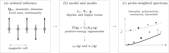
A defensible material analysis runs left to right: establish the ordered reference and magnetic cell, construct and stabilize the spin Hamiltonian, obtain positive-energy bosonic modes, and only then calculate the probe-weighted intensity. Energies constrain coupling combinations; intensities test eigenvectors, form factors, domains, and polarization.

Three Ordered Limits

Ferromagnets

An isotropic collinear ferromagnet has nonzero uniform spin density. Its two broken transverse generators form one canonical pair, giving one type-B Goldstone branch. At long wavelength,

$$\hbar\omega(\mathbf q) \simeq \Delta + D_{\alpha\beta}q_\alpha q_\beta.$$

The gap $\Delta$ vanishes only when the relevant continuous spin symmetry is exact and the field is zero. Crystalline anisotropy, dipolar interactions, and an applied field can gap or reshape the low-$q$ spectrum. Magnetic Anisotropy owns the easy-direction, demagnetizing, interface, and Dzyaloshinskii–Moriya energy ledger. A basis with several magnetic ions can add optical branches even though the phase has only one acoustic Goldstone mode.

The material definition, domain physics, and Curie behavior live in Ferromagnetism.

Antiferromagnets

In a simple collinear antiferromagnet, the leading order parameter lies at a nonzero ordering wavevector and the uniform spin density vanishes. Near a magnetic zone center, an isotropic continuum commonly gives linearly dispersing transverse modes:

$$\hbar\omega_\lambda(\mathbf q) \simeq \sqrt{ \Delta_\lambda^2 + c_{\lambda,\alpha\beta}^2 q_\alpha q_\beta }.$$

The branch or polarization index $\lambda$ matters when anisotropy or field splits the transverse modes. The same mode can be strong near one magnetic reciprocal vector and extinguished near another because the two sublattices interfere with different phases. A missing peak is therefore not automatically a missing eigenmode.

The material order parameter, magnetic unit cell, spin-flop response, and dimensional caveats live in Antiferromagnetism.

Ferrimagnets

A collinear ferrimagnet combines antiparallel sublattices with unequal moments. In the isotropic limit and away from angular-momentum compensation, the net spin density produces a quadratic acoustic mode, while relative motion of the sublattices produces an optical partner. Schematically,

$$\hbar\omega_{\mathrm{ac}}(\mathbf q) \sim Dq^2, \qquad \hbar\omega_{\mathrm{op}}(\mathbf 0) = \Delta_{\mathrm{op}} \gt 0.$$

The magnetization compensation temperature, angular-momentum compensation temperature, and Curie temperature are distinct. Near angular-momentum compensation, the gyrotropic coefficient of a coarse-grained description can become small and inertial, antiferromagnet-like dynamics become important. The detailed crossover depends on anisotropy, field, damping, and the retained sublattices; it is not a universal statement that every branch simply becomes linear.

Ferrimagnetism owns the sublattice ledger, compensation conditions, ferrite examples, and alternating-spin benchmark.

Multiple Sites, Noncollinearity, and Folding

A chemically complicated magnet can have many magnon branches without invoking exotic physics. If the magnetic primitive cell contains $n_m$ retained spins, harmonic theory generically produces $n_m$ positive-energy branches. Yttrium iron garnet is a standard warning: a large magnetic cell generates many branches, while only a subset may carry substantial weight in a given energy and momentum window.

Noncollinear order adds three complications:

1. every site needs its own local frame;
2. cubic interaction vertices can be symmetry allowed;
3. laboratory spin components mix several local transverse and longitudinal components.

These features can produce nonreciprocal dispersions, field-dependent mode hybridization, and spontaneous decay channels. They do not change the basic requirement that the ordered configuration be stationary before the expansion.

Zone folding is likewise a representation issue. A mode plotted in the chemical Brillouin zone may appear as several copies related by magnetic reciprocal vectors. To decide whether two peaks are independent branches, compare their periodicity, eigenvectors, and structure-factor weights in the magnetic zone.

What Inelastic Neutrons Measure

Define a dynamical spin correlation function by

$$S^{\alpha\beta}(\mathbf Q,\omega) = \frac{1}{2\pi N} \int_{-\infty}^{\infty} dt\, e^{i\omega t} \left\langle \hat S_{\mathbf Q}^{\alpha}(t) \hat S_{-\mathbf Q}^{\beta}(0) \right\rangle,$$

where

$$\hat S_{\mathbf Q}^{\alpha} = \sum_j e^{-i\mathbf Q\cdot\mathbf r_j} \hat S_j^\alpha.$$

Up to instrument and normalization conventions, the unpolarized magnetic neutron cross section has the form

$$\frac{d^2\sigma}{d\Omega\,dE_f} = C \frac{k_f}{k_i} \lvert F(\mathbf Q)\rvert^2 \sum_{\alpha\beta} \left( \delta_{\alpha\beta} - \widehat Q_\alpha\widehat Q_\beta \right) S^{\alpha\beta}(\mathbf Q,\omega).$$

The constant $C$ collects standard neutron and moment factors, and $F(\mathbf Q)$ is the magnetic form factor. The tensor

$$P_{\alpha\beta}(\widehat{\mathbf Q}) = \delta_{\alpha\beta} - \widehat Q_\alpha\widehat Q_\beta$$

projects out magnetic fluctuations parallel to $\mathbf Q$. Consequently, rotating the sample can make the same mode appear or disappear without changing its energy.

A one-magnon intensity also contains:

• the mode eigenvector and sublattice phase factors;
• the magnetic form factor of each ion;
• bosonic coherence factors;
• thermal occupation factors;
• domain and twin populations;
• instrumental resolution and background.

Plotting $\omega_\nu(\mathbf q)$ as a line over an intensity map tests only the peak positions. It does not test whether the model predicts the correct scattering operator matrix elements.

With the convention above, equilibrium detailed balance is

$$S^{\beta\alpha}(-\mathbf Q,-\omega) = e^{-\beta\hbar\omega} S^{\alpha\beta}(\mathbf Q,\omega).$$

For diagonal response in a reciprocal situation, the energy-gain side is therefore suppressed relative to the energy-loss side by $e^{-\beta\hbar\omega}$. This is both a physical population effect and a useful normalization check. Structure Factors and Time-Dependent Correlations own the general correlation-function conventions.

Other Spectroscopic Windows

No single probe measures a universal “magnon intensity.”

Neutron Scattering develops the instrument kinematics, polarization analysis, magnetic form factor, resolution convolution, normalization, and background controls behind the neutron row.

X-Ray Scattering develops the resonant intermediate-state, polarization, attenuation, and resolution controls behind the RIXS row.

Probe	Typical momentum window	What it is especially good at	Main interpretive caution
Inelastic neutron scattering	broad three-dimensional $\mathbf Q$ and energy coverage	bulk dispersions, polarizations, absolute spectral weight	sample volume, neutron absorption, form factors, resolution
Resonant inelastic x-ray scattering	finite momentum with element and edge selectivity	spin, orbital, charge, and lattice excitations in small samples and thin films	the resonant cross section is not generally identical to $S(\mathbf Q,\omega)$
Brillouin light scattering	very small wavevector and low energy	thin-film, surface, dipolar, and nonreciprocal modes	limited momentum range and optical selection rules
Raman scattering	near-zero photon momentum	symmetry-selected one- or multi-magnon channels	often probes composite operators rather than a single transverse spin
ESR, ferromagnetic resonance, and terahertz spectroscopy	near $\mathbf q=0$	gaps, field slopes, anisotropy, coherent mode dynamics	only modes with the required dipole matrix element are visible
Spin pumping and transport	device-dependent, often mode-integrated	driven populations, damping, propagation, interfaces	voltage or nonlocal signals are not direct spectral functions

Cross-probe agreement is powerful because different selection rules interrogate different pieces of the same eigenvectors. Cross-probe disagreement is not automatically a contradiction; first translate each measurement into its actual correlation function and geometry.

Fit the Forward Model

A robust analysis calculates the measured intensity from the Hamiltonian and experimental geometry:

$$I_{\mathrm{obs}}(\mathbf Q,\omega) = \int d\mathbf Q'\,d\omega'\, R( \mathbf Q-\mathbf Q', \omega-\omega' ) I_{\mathrm{model}}(\mathbf Q',\omega') + B(\mathbf Q,\omega).$$

Here $R$ is the instrumental resolution function and $B$ is a background model. Fitting unconvolved delta-function dispersions to broadened data can bias both energies and linewidths, especially near steep branches, crossings, or kinematic boundaries.

Energies and intensities constrain different things

Mode energies often constrain combinations of exchange parameters. Two different Hamiltonians can agree along a few high-symmetry cuts. Intensities add sensitivity to:

• the relative phases on inequivalent sites;
• eigenvector polarization;
• mode hybridization;
• magnetic form factors;
• domain populations.

This is why a fit to peak positions alone can be precise but not identifiable.

Use global constraints

Subject to the stated normalization and complete momentum and energy coverage, the total-moment sum rule has the schematic form

$$\frac{1}{N} \sum_{\mathbf Q} \int_{-\infty}^{\infty} d\omega \sum_\alpha S^{\alpha\alpha}(\mathbf Q,\omega) = S(S+1)$$

for one spin-$S$ degree of freedom per site. In a real material, covalency, multiple ions, orbital contributions, finite energy windows, and form-factor normalization must be included before using this as an absolute test. Partial spectral weight is not a violation of the sum rule if weight lies outside the measured window.

Other global checks include:

• symmetry-enforced degeneracies and periodicity;
• the correct number of magnetic domains;
• field slopes consistent with the stated $g$ tensors;
• gaps consistent with the symmetry broken explicitly by anisotropy or field;
• thermodynamic moments and ordering temperatures on compatible scales;
• stability of fitted parameters when additional momentum cuts are included.

Linewidths, Lifetimes, and Hybridization

The harmonic theory gives infinitely sharp poles. Interactions replace the bare pole by a dressed response. A schematic retarded Green function is

$$G_\nu^R(\mathbf q,\omega) = \frac{1}{ \hbar\omega - \varepsilon_{\nu0}(\mathbf q) - \Sigma_\nu^R(\mathbf q,\omega) }.$$

The real part of the self-energy shifts the mode, while the imaginary part broadens it. If an isolated peak is approximately Lorentzian and its energy full width at half maximum is $\Gamma_{\mathrm{FWHM}}$, an occupation lifetime is conventionally estimated as

$$\tau \simeq \frac{\hbar}{\Gamma_{\mathrm{FWHM}}}.$$

This estimate is meaningful only after deconvolving instrumental resolution and stating the linewidth convention. A non-Lorentzian asymmetric line, an unresolved doublet, or a branch crossing should not be compressed into a single lifetime without a model.

Magnons can broaden through:

• magnon–magnon scattering;
• magnon–phonon hybridization and decay;
• coupling to electron–hole or Stoner continua;
• disorder and domain boundaries;
• finite-temperature scattering;
• coupling to other crystal-field or orbital excitations.

An avoided crossing with exchange of spectral weight is evidence for hybridization, not merely two dispersions passing nearby. The coupled-mode eigenvectors should rotate through the crossing, and both energies and intensities should be fitted.

When the Magnon Description Fails

A sharp dispersing peak is strong evidence for a quasiparticle when its linewidth is small compared with its energy and nearby spectral scales. The converse is not automatic: a broad magnetic continuum can come from interacting magnons, fractional excitations, disorder, itinerant particle–hole pairs, or unresolved branches.

Audit the magnon description when:

1. $\Gamma_{\mathrm{FWHM}}$ becomes comparable to the excitation energy;
2. the fitted pole loses most of its spectral residue;
3. a continuum carries substantial weight where harmonic theory predicts only one mode;
4. the assumed ordered state is absent or strongly fluctuating;
5. the local-moment sum rule and field response are incompatible with the fitted spins;
6. the mode enters a symmetry- and kinematically allowed decay continuum;
7. a one-dimensional or quantum-disordered system has elementary excitations other than magnons.

Energy and momentum conservation are necessary for decay, but not sufficient. The interaction vertex and all symmetry selection rules must also be nonzero. Conversely, a sharp mode inside a naive two-particle continuum can remain stable because the relevant coupling vanishes.

Worked Material Inference: Simple-Cubic Ferromagnet

Consider the explicitly defined model

$$\hat H = - J \sum_{\langle ij\rangle} \hat{\mathbf S}_i\cdot\hat{\mathbf S}_j - g\mu_B B \sum_i \hat S_i^z, \qquad J\gt0,$$

with one dimensionless spin $S$ per simple-cubic cell of lattice constant $a$. Linear spin-wave theory gives

$$\begin{aligned} \varepsilon(\mathbf q) ={}& g\mu_B B \\ &+ 2JS \left[ 3 - \cos(q_xa) - \cos(q_ya) - \cos(q_za) \right]. \end{aligned}$$

Near $\mathbf q=\mathbf 0$,

$$\varepsilon(\mathbf q) \simeq \Delta + Dq^2, \qquad \Delta=g\mu_B B, \qquad D=JSa^2.$$

At the $X$ point $\mathbf q_X=(\pi/a,0,0)$,

$$\varepsilon_X = \Delta+4JS.$$

Therefore two directly interpretable estimates are

$$J = \frac{\varepsilon_X-\Delta}{4S}, \qquad D_{\mathrm{pred}} = \frac{\varepsilon_X-\Delta}{4}a^2.$$

The second relation is a falsifiable consistency check. If the measured low-$q$ stiffness disagrees with the value predicted from the zone boundary, the nearest-neighbor model is incomplete. Further-neighbor exchange, dipolar terms, anisotropy, itinerancy, or energy-dependent renormalization may be required. Adding parameters is justified only after identifying which additional measurements separate those possibilities.

Common Mistakes

Treating a spin wave and a one-magnon state as identical

A coherent spin wave has a definite phase and transverse expectation value. A one-magnon number eigenstate has a definite occupation but generally no classical transverse mean. The canonical Magnons page gives the operator-level distinction.

Fitting only a line drawing

Peak energies do not test sublattice phases, polarization, domains, or form factors. Calculate the cross section and resolution-convolved intensity.

Using the chemical Brillouin zone without a magnetic-cell ledger

Magnetic order folds the zone. State whether every momentum is reduced in the chemical or magnetic reciprocal lattice.

Reading an intensity zero as an absent mode

Polarization projection, sublattice interference, form-factor suppression, or the selected probe operator can extinguish a real eigenmode.

Reporting exchange constants without the Hamiltonian

The sign, factor of two, bond multiplicity, and spin normalization vary across communities and software.

Calling every broad magnetic feature a magnon

A quasiparticle requires an identifiable pole or controlled resonance. Continua demand tests against multi-magnon, fractional, itinerant, disorder, and hybridization mechanisms.

Interpreting fitted precision as parameter identifiability

Small statistical error bars do not resolve degeneracies built into a restricted momentum path or an incomplete forward model.

Ignoring temperature and resolution

Thermal populations, self-energy shifts, domain changes, and instrumental convolution can all move or broaden apparent peaks.

Exercises

Exercise 1: Branch count versus Goldstone count

A collinear ferromagnet has two magnetic ions in its magnetic primitive cell. The ions are equivalent by a nonsymmorphic symmetry, and the Hamiltonian is isotropic at zero field.

1. How many positive-energy harmonic branches are generically present?
2. How many acoustic Goldstone branches are required by the broken spin symmetry?
3. Why need the two answers not agree?

Solution

There is one Holstein–Primakoff boson per retained magnetic ion, so the generic harmonic problem has two positive-energy branches. Symmetry can force degeneracies, but it does not remove the two-dimensional positive-frequency mode space.

The ferromagnet has one type-B Goldstone branch. The two broken transverse spin generators form one canonical pair because their commutator has a nonzero expectation value proportional to the uniform magnetization.

The second branch describes relative motion within the magnetic basis and is generally optical and gapped. Branch count follows the magnetic basis; Goldstone count follows broken symmetries and their commutator algebra.

Exercise 2: Extract exchange and test stiffness

For the simple-cubic model above, let

$$S=1, \qquad a=0.40\,\mathrm{nm}, \qquad \Delta=0.20\,\mathrm{meV}, \qquad \varepsilon_X=8.20\,\mathrm{meV}.$$

Find $J$ and the predicted stiffness $D$.

Solution

The exchange follows from

$$J = \frac{8.20-0.20}{4\times1}\,\mathrm{meV} = 2.00\,\mathrm{meV}.$$

Then

$$\begin{aligned} D &= JSa^2 \\ &= (2.00\,\mathrm{meV}) (1) (0.40\,\mathrm{nm})^2 \\ &= 0.32\,\mathrm{meV\,nm^2}. \end{aligned}$$

A measured low-$q$ stiffness inconsistent with this value would falsify the nearest-neighbor model even if it reproduced $\varepsilon_X$.

Exercise 3: Neutron polarization extinction

Suppose a mode fluctuates entirely along laboratory $\hat{\mathbf z}$. Compare its unpolarized neutron intensity for $\mathbf Q\parallel\hat{\mathbf z}$ and $\mathbf Q\parallel\hat{\mathbf x}$, ignoring form factors and all other geometry.

Solution

The relevant factor is

$$P_{zz} = 1-\widehat Q_z^2.$$

For $\mathbf Q\parallel\hat{\mathbf z}$, $\widehat Q_z=1$ and $P_{zz}=0$, so the fluctuation is extinguished. For $\mathbf Q\parallel\hat{\mathbf x}$, $\widehat Q_z=0$ and $P_{zz}=1$, so it is fully visible within the stated simplifications.

The eigenmode exists in both geometries. Only its projection into the neutron cross section changes.

Exercise 4: Detailed-balance check

At $T=100\,\mathrm K$, a reciprocal magnetic excitation has energy $\hbar\omega=10\,\mathrm{meV}$. What is the equilibrium ratio of the energy-gain intensity to the energy-loss intensity?

Use $k_B=0.08617\,\mathrm{meV/K}$.

Solution

Detailed balance gives

$$\frac{I(-\omega)}{I(+\omega)} = \exp\left( - \frac{\hbar\omega}{k_BT} \right).$$

Here

$$k_BT = 8.617\,\mathrm{meV},$$

so

$$\frac{I(-\omega)}{I(+\omega)} = e^{-10/8.617} \simeq 0.313.$$

A substantially different ratio calls for an audit of background subtraction, detector normalization, the sign convention for energy transfer, or nonequilibrium driving.

Exercise 5: Linewidth and lifetime convention

An isolated magnon at $12\,\mathrm{meV}$ has a deconvolved Lorentzian energy FWHM of $1.2\,\mathrm{meV}$. Estimate its lifetime using $\hbar=0.6582\,\mathrm{meV\,ps}$ and calculate the ratio of energy to FWHM.

Solution

With the FWHM convention used on this page,

$$\tau \simeq \frac{\hbar}{\Gamma_{\mathrm{FWHM}}} = \frac{0.6582\,\mathrm{meV\,ps}} {1.2\,\mathrm{meV}} \simeq 0.55\,\mathrm{ps}.$$

The energy-to-width ratio is

$$\frac{\varepsilon}{\Gamma_{\mathrm{FWHM}}} = \frac{12}{1.2} = 10.$$

This is a reasonably resolved resonance, but not an infinitely sharp harmonic pole. Quoting a lifetime without saying whether the reported width is a half width or full width would introduce a factor-of-two ambiguity.

Exercise 6: Diagnose a partial fit

A four-parameter local-spin model reproduces all observed peak energies along one high-symmetry line. It predicts a strong optical branch at a second reciprocal vector, but no peak is observed there. Give a controlled diagnostic sequence before discarding the branch.

Solution

First compute the full probe intensity, including the mode eigenvector, sublattice phase factors, polarization projector, ion-specific form factors, domain populations, thermal factor, and instrumental resolution. The branch may be extinguished in that geometry.

Second inspect symmetry-related reciprocal vectors and rotate the polarization geometry. A genuine mode with a selection-rule zero at one $\mathbf Q$ can become visible elsewhere.

Third check whether the predicted branch overlaps another excitation, background, or a region of poor resolution. Fit a resolution-convolved two-mode or coupled-mode model rather than a single peak.

Fourth test for damping or hybridization by looking for redistributed spectral weight, an avoided crossing, or a continuum. Only after these checks should the missing intensity be used to reject the Hamiltonian or the assumed magnetic structure.

Connections

• Magnetic Moments in Matter validates the retained moment manifold and elastic–inelastic moment budget before this page constructs and tests a material spin-wave forward model.
• Magnons is the canonical home for Holstein–Primakoff quantization, bosonic Bogoliubov theory, mode quantum numbers, interactions, and breakdown.
• Exchange Interactions derives the microscopic pathways that become material spin couplings.
• RKKY Interaction derives the long-range oscillatory exchange network whose Fourier transform can select helical or incommensurate modes.
• Ferromagnetism owns uniform order, domains, Curie behavior, and the material interpretation of quadratic acoustic modes.
• Antiferromagnetism owns Néel order, magnetic unit cells, spin flop, frustration, and quantum reduction.
• Ferrimagnetism owns unequal opposing sublattices, compensation points, ferrites, and acoustic–optical mode pairing.
• Spintronics owns the device-level spin-pumping, inverse-conversion, nonlocal-transport, and torque ledger used to launch and detect magnetic dynamics.
• Skyrmions and Magnetic Textures develops walls, vortices, skyrmions, their internal modes, and the limits of a rigid-texture description.
• Itinerant Magnetism explains susceptibility poles, Stoner electron–hole continua, and when a local-spin spectrum is only an effective parametrization.
• Structure Factors develops static and dynamic scattering conventions.
• Fluctuation–Dissipation Theorem relates equilibrium response and correlation spectra.
• Goldstone Modes in Many-Body Systems gives type-A and type-B counting independent of microscopic branch multiplicity.
• Phonons provides the parallel normal-mode language and the material setting for magnon–phonon hybridization.
• Reciprocal Lattice and Brillouin Zones fix the momentum-space geometry used in scattering maps.

References

1. F. Bloch, “Zur Theorie des Ferromagnetismus,” Zeitschrift für Physik 61, 206–219 (1930), doi:10.1007/BF01339661.
2. T. Holstein and H. Primakoff, “Field Dependence of the Intrinsic Domain Magnetization of a Ferromagnet,” Physical Review 58, 1098–1113 (1940), doi:10.1103/PhysRev.58.1098.
3. C. Herring and C. Kittel, “On the Theory of Spin Waves in Ferromagnetic Media,” Physical Review 81, 869–880 (1951), doi:10.1103/PhysRev.81.869.
4. P. W. Anderson, “An Approximate Quantum Theory of the Antiferromagnetic Ground State,” Physical Review 86, 694–701 (1952), doi:10.1103/PhysRev.86.694.
5. R. Kubo, “The Spin-Wave Theory of Antiferromagnetics,” Physical Review 87, 568–580 (1952), doi:10.1103/PhysRev.87.568.
6. F. J. Dyson, “General Theory of Spin-Wave Interactions,” Physical Review 102, 1217–1230 (1956), doi:10.1103/PhysRev.102.1217.
7. P. A. Fleury and R. Loudon, “Scattering of Light by One- and Two-Magnon Excitations,” Physical Review 166, 514–530 (1968), doi:10.1103/PhysRev.166.514.
8. G. L. Squires, Introduction to the Theory of Thermal Neutron Scattering, 3rd ed. (Cambridge University Press, 2012), doi:10.1017/CBO9781139107808.
9. A. Auerbach, Interacting Electrons and Quantum Magnetism (Springer, 1994), doi:10.1007/978-1-4612-0869-3.
10. R. L. Stamps et al., “The 2014 Magnetism Roadmap,” Journal of Physics D: Applied Physics 47, 333001 (2014), doi:10.1088/0022-3727/47/33/333001.
11. A. V. Chumak, V. I. Vasyuchka, A. A. Serga, and B. Hillebrands, “Magnon Spintronics,” Nature Physics 11, 453–461 (2015), doi:10.1038/nphys3347.
12. V. Cherepanov, I. Kolokolov, and V. L’vov, “The Saga of YIG: Spectra, Thermodynamics, Interaction and Relaxation of Magnons in a Complex Magnet,” Physics Reports 229, 81–144 (1993), doi:10.1016/0370-1573(93)90107-O.
13. S. O. Bayrakci, T. Keller, K. Habicht, and B. Keimer, “Spin-Wave Lifetimes throughout the Brillouin Zone,” Science 312, 1926–1929 (2006), doi:10.1126/science.1127756.
14. L. J. P. Ament, M. van Veenendaal, T. P. Devereaux, J. P. Hill, and J. van den Brink, “Resonant Inelastic X-Ray Scattering Studies of Elementary Excitations,” Reviews of Modern Physics 83, 705–767 (2011), doi:10.1103/RevModPhys.83.705.
15. M. E. Zhitomirsky and A. L. Chernyshev, “Colloquium: Spontaneous Magnon Decays,” Reviews of Modern Physics 85, 219–242 (2013), doi:10.1103/RevModPhys.85.219.
16. S. O. Bayrakci et al., “Lifetimes of Antiferromagnetic Magnons in Two and Three Dimensions: Experiment, Theory, and Numerics,” Physical Review Letters 111, 017204 (2013), doi:10.1103/PhysRevLett.111.017204.