Fluctuation–Dissipation Theorem

The fluctuation–dissipation theorem states that thermal-equilibrium fluctuations and linear dissipative response are two spectral combinations of the same transitions. The ordered correlation spectrum counts thermally weighted transition strength. The absorptive susceptibility counts absorption minus the thermally reversed process. Equilibrium detailed balance fixes the ratio of those two directions, so either fluctuation data or dissipative response determines the other.

For a Hermitian observable $A$, one familiar angular-frequency form is

$$S_{AA}^{\mathrm{sym}}(\omega) = \hbar \coth\left( \frac{\beta\hbar\omega}{2} \right) \operatorname{Im} \chi_{AA}^{\mathrm R}(\omega),$$

under the source, Fourier, and spectral conventions stated below. The hyperbolic cotangent is not a decorative quantum correction. It encodes the Kubo–Martin–Schwinger, or KMS, balance between a thermal system absorbing and releasing energy.

The theorem is exact for equilibrium linear response. It is not a general identity for an arbitrary stationary, noisy, driven, or open state.

Canonical Scope

This page is the canonical home for the many-body equilibrium fluctuation–dissipation theorem. It owns:

• the assumptions under which the theorem holds;
• the KMS and Lehmann derivation of detailed balance;
• ordered, reversed, commutator, and symmetrized spectral conventions;
• the quantum Bose factor and its classical high-temperature limit;
• the zero-temperature and zero-frequency limits;
• the distinction between dynamic fluctuations and static thermodynamic covariance;
• matrix and momentum-resolved forms;
• harmonic-oscillator and two-level benchmarks;
• numerical, experimental, and approximation checks.

Neighboring pages retain separate ownership:

• KMS Condition Preview owns the finite Gibbs derivation, analytic strip, imaginary-time boundary relation, stationarity test, and algebraic equilibrium bridge.
• Time-Dependent Correlations owns ordinary two-time correlators, their Lehmann representation, and a bounded KMS preview.
• Retarded and Advanced Response owns causal support, analytic boundary values, response spectral density, and dispersion relations.
• Spectral Representation owns the common thermal Lehmann construction, Euclidean kernels, Matsubara transforms, retarded bridge, and static bosonic term.
• Kubo Formula owns the source-coupled derivation of linear response, contact terms, conductivity, and order-of-limits cautions.
• Spectral Functions owns line shapes, quasiparticle criteria, linewidths, spectral weight, and measured-intensity forward models.
• Fluctuations and Susceptibilities owns static equilibrium Hessians, Kubo–Mori covariance, and ensemble-dependent fluctuation identities.
• Fluctuation–Dissipation Relation owns bath-noise, damping-kernel, transition-rate, Johnson–Nyquist, and open-system applications.
• Sum Rules owns the exact spectral-moment and nested-commutator hierarchy.
• Transport Coefficients Preview owns Green–Kubo integrals, diffusion, viscosity, and the ballistic-versus-dissipative distinction.

This page derives the theorem for equilibrium observables. Fermionic lesser and greater single-particle Green functions have related KMS identities with Fermi occupation factors; their conventions belong to Green Functions in Many-Body QM.

Assumptions of the Theorem

The equilibrium theorem requires more than stationarity.

1. Thermal equilibrium. The reference state is a Gibbs or grand-canonical Gibbs state for the generator used in time evolution.
2. Stationarity. Correlations depend on a time difference, so a one-frequency representation exists.
3. Linear response. The source is weak enough that first-order response is meaningful.
4. Conjugate source. The perturbation and the susceptibility use the same declared source coupling.
5. Compatible orderings. Ordered, reversed, commutator, and symmetrized spectra are built from the same operator pair.
6. Compatible conventions. Fourier signs, factors of $\hbar$ and $2\pi$, and the meaning of positive energy are held fixed.
7. Well-defined transforms. Correlators are distributions or sufficiently regular functions for the spectral manipulations being used.

Time-reversal symmetry is not required for the basic equilibrium theorem. Time reversal enters reciprocity relations between different channels, not the KMS balance that follows from a Gibbs state.

Convention Ledger

Thermal generator

Write the equilibrium state as

$$\rho_\beta = \frac{ e^{-\beta\mathcal K} }{ \mathcal Z }, \qquad \mathcal Z = \operatorname{Tr} e^{-\beta\mathcal K}.$$

For a canonical ensemble,

$$\mathcal K = H.$$

For a grand-canonical ensemble,

$$\mathcal K = H-\mu\hat N.$$

Operators evolve with the same generator:

$$A(t) = e^{i\mathcal Kt/\hbar} A e^{-i\mathcal Kt/\hbar}.$$

For number-preserving observables, evolution with $H$ or $H-\mu\hat N$ is identical. For a number-changing operator, the distinction shifts the spectral energy by the appropriate chemical work. Mixing the two generators changes the detailed-balance exponent.

Connected operators

Define

$$\delta A = A-\langle A\rangle_\beta, \qquad \delta B = B-\langle B\rangle_\beta.$$

Subtracting the means removes the trivial elastic line produced by one-point functions. It does not remove every zero-energy contribution: conserved projections and exact degeneracies can still produce singular weight at $E=0$.

The commutator is unchanged by this subtraction, but the fluctuation spectrum is not.

Positive energy

The spectral variable is the target energy transfer

$$E = \hbar\omega.$$

Positive $E$ means that the equilibrium target absorbs energy from the source or probe. Negative $E$ describes the thermally reversed direction.

Ordered spectra

Define

$$\begin{aligned} \mathcal S_{AB}^{>}(E) ={}& \frac{1}{2\pi\hbar} \int_{-\infty}^{\infty} dt\, e^{iEt/\hbar} \\ &\times \left\langle \delta A(t) \delta B(0) \right\rangle_\beta, \end{aligned}$$

and

$$\begin{aligned} \mathcal S_{AB}^{<}(E) ={}& \frac{1}{2\pi\hbar} \int_{-\infty}^{\infty} dt\, e^{iEt/\hbar} \\ &\times \left\langle \delta B(0) \delta A(t) \right\rangle_\beta. \end{aligned}$$

For a Hermitian autochannel, set $B=A$ and abbreviate these as $\mathcal S_A^{>}$ and $\mathcal S_A^{<}$. They obey

$$\mathcal S_A^{<}(E) = \mathcal S_A^{>}(-E).$$

With this normalization,

$$\int_{-\infty}^{\infty} dE\, \mathcal S_A^{>}(E) = \left\langle (\delta A)^2 \right\rangle_\beta.$$

Retarded response

Use the source convention

$$H_{\mathrm{pert}}(t) = -f(t)B.$$

The retarded susceptibility is

$$\chi_{AB}^{\mathrm R}(t) = \frac{i}{\hbar} \theta(t) \left\langle [ \delta A(t), \delta B(0) ] \right\rangle_\beta.$$

Its energy-domain transform is

$$\chi_{AB}^{\mathrm R}(E) = \int_{-\infty}^{\infty} dt\, e^{iEt/\hbar} \chi_{AB}^{\mathrm R}(t).$$

Write

$$\chi_{AB}'(E) = \operatorname{Re} \chi_{AB}^{\mathrm R}(E), \qquad \chi_{AB}''(E) = \operatorname{Im} \chi_{AB}^{\mathrm R}(E).$$

For a Hermitian autochannel and $E\gt0$, passivity gives

$$\chi_{AA}''(E) \geq 0$$

with these conventions.

Dissipated power

Let

$$f(t) = \operatorname{Re} \left( f_0 e^{-i\omega t} \right), \qquad \omega\gt0.$$

The cycle-averaged work delivered to the system is

$$\overline P = \frac{\omega}{2} \lvert f_0\rvert^2 \chi_{AA}''(\omega).$$

Thus $\chi''$ is the absorptive part for the declared source sign. Reversing the sign in the retarded definition or source coupling reverses intermediate signs, but a passive system must still absorb nonnegative average power.

The Theorem in Energy Form

Define the response spectral density

$$\rho_{AB}(E) = \mathcal S_{AB}^{>}(E) - \mathcal S_{AB}^{<}(E).$$

Thermal equilibrium gives detailed balance:

$$\mathcal S_{AB}^{<}(E) = e^{-\beta E} \mathcal S_{AB}^{>}(E).$$

Therefore

$$\rho_{AB}(E) = \left( 1-e^{-\beta E} \right) \mathcal S_{AB}^{>}(E).$$

For the retarded convention above,

$$\chi_{AB}''(E) = \pi \rho_{AB}(E).$$

The ordered form of the theorem is consequently

$$\mathcal S_{AB}^{>}(E) = \frac{ \chi_{AB}''(E) }{ \pi \left( 1-e^{-\beta E} \right) }.$$

For a Hermitian autochannel, define the symmetrized spectrum

$$\mathcal S_A^{\mathrm{sym}}(E) = \frac12 \left[ \mathcal S_A^{>}(E) + \mathcal S_A^{<}(E) \right].$$

Combining the preceding relations gives

$$\mathcal S_A^{\mathrm{sym}}(E) = \frac{1}{2\pi} \coth\left( \frac{\beta E}{2} \right) \chi_{AA}''(E).$$

Equivalently,

$$\begin{aligned} \mathcal S_A^{>}(E) &= \left[ 1+n_{\mathrm B}(E) \right] \rho_{AA}(E), \\ \mathcal S_A^{<}(E) &= n_{\mathrm B}(E) \rho_{AA}(E), \end{aligned}$$

for $E\gt0$, where

$$n_{\mathrm B}(E) = \frac{1}{ e^{\beta E}-1 }.$$

The Bose factor appears because an observable response compares transitions differing by an energy $E$. It does not assert that the microscopic constituents are bosons.

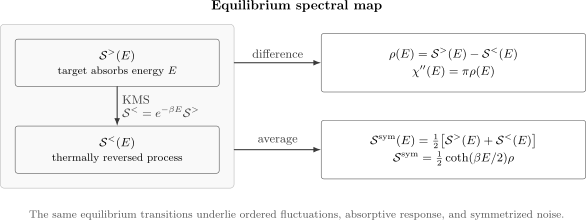
At equilibrium, KMS detailed balance fixes the reversed ordered spectrum from the forward one. Their difference is the response spectral density and hence the absorptive susceptibility; their average is the symmetrized fluctuation spectrum. The hyperbolic-cotangent factor is the ratio of that average to that difference.

Angular-Frequency Dictionary

Many texts omit the $1/(2\pi\hbar)$ factor and use angular frequency directly:

$$\begin{aligned} S_{AA}^{\mathrm{sym}}(\omega) ={}& \frac12 \int_{-\infty}^{\infty} dt\, e^{i\omega t} \\ &\times \left\langle \{ \delta A(t), \delta A(0) \} \right\rangle_\beta. \end{aligned}$$

The relation between the two conventions is

$$S_{AA}^{\mathrm{sym}}(\omega) = 2\pi\hbar\, \mathcal S_A^{\mathrm{sym}} \left( \hbar\omega \right).$$

Therefore the same theorem becomes

$$S_{AA}^{\mathrm{sym}}(\omega) = \hbar \coth\left( \frac{\beta\hbar\omega}{2} \right) \chi_{AA}''(\omega).$$

The unnormalized ordered spectrum

$$S_{AA}^{>}(\omega) = \int dt\, e^{i\omega t} \left\langle \delta A(t)\delta A(0) \right\rangle_\beta$$

obeys

$$S_{AA}^{>}(\omega) = \frac{ 2\hbar }{ 1-e^{-\beta\hbar\omega} } \chi_{AA}''(\omega).$$

These formulas are equivalent to the energy-normalized forms. Combining a spectrum from one convention with a susceptibility from another produces exactly the stray factors of $\hbar$, $2\pi$, and $\pi$ that frequently appear in incorrect comparisons.

Lehmann and KMS Derivation

Let

$$\mathcal K \lvert n\rangle = \kappa_n \lvert n\rangle, \qquad p_n = \frac{ e^{-\beta\kappa_n} }{ \mathcal Z }.$$

Insert a complete set of eigenstates into the ordered spectrum:

$$\begin{aligned} \mathcal S_{AB}^{>}(E) ={}& \sum_{n,m} p_n (\delta A)_{nm} (\delta B)_{mn} \\ &\times \delta \left( E-\kappa_m+\kappa_n \right). \end{aligned}$$

The reversed order gives

$$\begin{aligned} \mathcal S_{AB}^{<}(E) ={}& \sum_{n,m} p_m (\delta A)_{nm} (\delta B)_{mn} \\ &\times \delta \left( E-\kappa_m+\kappa_n \right). \end{aligned}$$

On the support of the delta function,

$$\kappa_m-\kappa_n = E,$$

so

$$\frac{p_m}{p_n} = e^{-\beta E}.$$

Term by term,

$$\mathcal S_{AB}^{<}(E) = e^{-\beta E} \mathcal S_{AB}^{>}(E).$$

This is frequency-domain KMS detailed balance. It follows from the Gibbs weights and cyclicity of the trace, not from weak interactions, a quasiparticle approximation, chaos, or a thermodynamic limit.

The corresponding time-domain identity is

$$\left\langle \delta A(t)\delta B(0) \right\rangle_\beta = \left\langle \delta B(0) \delta A(t+i\beta\hbar) \right\rangle_\beta,$$

when the analytic continuation and operator domains are well defined.

From the commutator to absorption

The commutator spectrum is

$$\rho_{AB}(E) = \mathcal S_{AB}^{>}(E) - \mathcal S_{AB}^{<}(E).$$

The retarded spectral representation can be written as

$$\chi_{AB}^{\mathrm R}(E) = \int_{-\infty}^{\infty} dE'\, \frac{ \rho_{AB}(E') }{ E'-E-i0^+ }.$$

The distributional identity

$$\frac{1}{ x-i0^+ } = \operatorname{PV} \frac{1}{x} + i\pi\delta(x)$$

then gives

$$\chi_{AB}''(E) = \pi\rho_{AB}(E).$$

The theorem follows by combining this response identity with detailed balance.

Charged operators and chemical work

Suppose the state is grand canonical but operators are evolved with the physical Hamiltonian $H$. If a transition changes particle number by $\Delta N$, then the Gibbs-weight ratio is

$$\frac{p_m}{p_n} = \exp \left[ -\beta \left( E-\mu\Delta N \right) \right].$$

The detailed-balance exponent is therefore the change in

$$H-\mu\hat N,$$

not the physical energy alone. Evolving with $\mathcal K=H-\mu\hat N$ packages this chemical work into the spectral variable. A number-changing spectrum must state which choice is being used.

What Fluctuation and Dissipation Mean

The theorem combines three different spectral operations.

Forward ordered spectrum

For $E\gt0$,

$$\mathcal S_A^{>}(E)$$

counts thermally weighted transitions in which the target gains energy $E$. It is nonnegative for a Hermitian autochannel.

Reversed ordered spectrum

The reversed process is

$$\mathcal S_A^{<}(E) = e^{-\beta E} \mathcal S_A^{>}(E).$$

At low temperature it is suppressed because the target must begin in an excited state to release the same energy.

Dissipative difference

The absorptive response is proportional to

$$\mathcal S_A^{>}(E) - \mathcal S_A^{<}(E).$$

Stimulated emission subtracts from absorption. This is why a highly populated excited transition can reduce or reverse dissipation.

Symmetrized average

The symmetrized spectrum is proportional to

$$\mathcal S_A^{>}(E) + \mathcal S_A^{<}(E).$$

It records both directions without identifying which one can excite a detector. A nonzero zero-temperature symmetrized spectrum is therefore compatible with the absence of negative-energy emission from a ground-state target.

Temperature Regimes

Classical high-temperature limit

When

$$\beta\lvert E\rvert \ll 1,$$

the thermal factor is

$$\coth\left( \frac{\beta E}{2} \right) = \frac{2}{\beta E} + O(\beta E).$$

The energy-normalized theorem becomes

$$\mathcal S_A^{\mathrm{sym}}(E) \simeq \frac{ k_{\mathrm B}T }{ \pi E } \chi_{AA}''(E).$$

In angular-frequency notation,

$$S_{AA}^{\mathrm{sym}}(\omega) \simeq \frac{ 2k_{\mathrm B}T }{ \omega } \chi_{AA}''(\omega).$$

The classical limit requires

$$\hbar\lvert\omega\rvert \ll k_{\mathrm B}T$$

at the frequency being examined. A system can be classical at low frequency and quantum at high frequency at the same temperature.

For a classical equilibrium variable with correlation

$$C_A(t) = \left\langle \delta A(t)\delta A(0) \right\rangle,$$

the time-domain form is

$$\chi_{AA}^{\mathrm R}(t) = -\beta \theta(t) \frac{dC_A(t)}{dt},$$

under the same source sign. The fully quantum analogue uses a Kubo-transformed imaginary-time correlation rather than the ordinary product.

Quantum low-temperature limit

At fixed nonzero energy,

$$\beta\lvert E\rvert \gg 1.$$

Then

$$\coth\left( \frac{\beta E}{2} \right) \longrightarrow \operatorname{sgn}(E).$$

For $E\gt0$,

$$\mathcal S_A^{<}(E) \longrightarrow 0,$$

while

$$\mathcal S_A^{>}(E) \longrightarrow \rho_{AA}(E).$$

The symmetrized spectrum retains half of the positive- and negative-energy pair:

$$\mathcal S_A^{\mathrm{sym}}(E) \longrightarrow \frac{1}{2\pi} \left| \chi_{AA}''(E) \right|.$$

This is often called zero-point fluctuation. It does not mean that a ground-state target can supply positive energy to another system.

Infinite-temperature limit

For a finite-dimensional system,

$$\beta \longrightarrow 0$$

makes thermal populations equal. Then absorption and stimulated emission approach one another:

$$\rho_{AA}(E) = O(\beta E).$$

The symmetrized fluctuation spectrum can remain finite even though the net dissipative difference vanishes. Large fluctuations and weak net absorption are therefore compatible.

The Zero-Frequency Limit

The factor

$$\coth\left( \frac{\beta E}{2} \right)$$

diverges as $E\to0$, while a regular passive response has

$$\chi_{AA}''(E) = O(E).$$

Their product can have a finite limit. One should therefore evaluate

$$\lim_{E\to0} \frac{ \chi_{AA}''(E) }{ E },$$

not substitute $E=0$ into the factors separately.

Singular cases require more care:

• an exactly conserved operator can produce a delta function at $E=0$;
• ballistic transport can contain a Drude contribution;
• spontaneous symmetry breaking can make the thermodynamic and dynamic limits noncommuting;
• diffusion produces a pole whose form depends on the order of $E\to0$ and $\mathbf q\to0$;
• finite systems retain exact zero-energy transitions inside degenerate subspaces.

The fluctuation–dissipation theorem remains a distributional relation, but dividing distributions by $E$ without a limiting prescription is not legitimate.

Dynamic Versus Static Fluctuation Relations

The dynamic theorem should not be shortened to

$$\chi(0) = \beta \operatorname{Var}(A)$$

for an arbitrary quantum observable.

The static isothermal susceptibility for

$$H_f = H_0-fA$$

is

$$\chi_T = \left. \frac{ \partial\langle A\rangle_f }{ \partial f } \right|_{f=0}.$$

Its exact equilibrium form is

$$\chi_T = \int_0^\beta d\lambda\, \left\langle \delta A(-i\hbar\lambda) \delta A(0) \right\rangle_\beta.$$

This is $\beta$ times the Kubo–Mori covariance. If

$$[ A,H_0 ] = 0,$$

the imaginary-time operator is constant and

$$\chi_T = \beta \operatorname{Var}(A).$$

Otherwise the ordinary variance and the static response differ.

The same distinction follows spectrally. A zero-frequency dispersion relation gives, when convergence and limit conditions hold,

$$\chi_{AA}'(0) = \operatorname{PV} \int_{-\infty}^{\infty} dE\, \frac{ \rho_{AA}(E) }{ E }.$$

Using detailed balance,

$$\chi_{AA}'(0) = \operatorname{PV} \int dE\, \frac{ 1-e^{-\beta E} }{ E } \mathcal S_A^{>}(E).$$

The energy-dependent factor is not generally the constant $\beta$. Fluctuations and Susceptibilities develops the static Kubo–Mori identity and its thermodynamic consequences.

Contact terms, constrained ensembles, and the order of uniform and static limits can further distinguish a measured susceptibility from $\chi_{AA}'(0)$. Those protocol choices belong to Susceptibilities and the Kubo Formula.

Matrix and Cross-Channel Form

Let a physical source couple to

$$B_v = \sum_a v_a B_a,$$

and let the conjugate detector be

$$A_v = B_v^\dagger.$$

For every channel vector $v$, the scalar spectrum obeys

$$\mathcal S_v^{<}(E) = e^{-\beta E} \mathcal S_v^{>}(E),$$

and

$$\mathcal S_v^{\mathrm{sym}}(E) = \frac{1}{2\pi} \coth\left( \frac{\beta E}{2} \right) \chi_v''(E).$$

This quadratic-form statement is safer than asserting componentwise positivity. Off-diagonal cross spectra and cross susceptibilities can be complex. Their Hermitian-conjugation, index-reversal, and time-reversal properties must be handled before reducing the theorem to separate real components.

KMS detailed balance still holds without time-reversal symmetry. Onsager–Casimir reciprocity is an additional statement involving operator parities and reversal of magnetic fields or other time-reversal-odd controls.

Momentum-Resolved Form

For a Hermitian local density or spin field,

$$O_{\mathbf q}^{\dagger} = O_{-\mathbf q}.$$

Define the ordered structure factor

$$\begin{aligned} S_O(\mathbf q,E) \propto{}& \int dt\, e^{iEt/\hbar} \\ &\times \left\langle \delta O_{\mathbf q}(t) \delta O_{-\mathbf q}(0) \right\rangle_\beta, \end{aligned}$$

with the volume and Fourier normalization declared separately. Detailed balance is

$$S_O(\mathbf q,-E) = e^{-\beta E} S_O(-\mathbf q,E).$$

Only when symmetry or reciprocity permits

$$S_O(\mathbf q,E) = S_O(-\mathbf q,E)$$

may one write the same-$\mathbf q$ shortcut

$$S_O(\mathbf q,-E) = e^{-\beta E} S_O(\mathbf q,E).$$

The corresponding density or spin response obeys, in compatible normalization,

$$\chi_O''(\mathbf q,E) \propto \left( 1-e^{-\beta E} \right) S_O(\mathbf q,E).$$

This relation connects scattering intensity to absorptive response. Probe form factors, polarization projectors, detector efficiency, and resolution still belong to the experimental forward model; they are not part of the intrinsic theorem.

Worked Benchmark: Harmonic Oscillator

Consider

$$H = \hbar\omega_0 \left( a^\dagger a+\frac12 \right)$$

and

$$x = \sqrt{ \frac{\hbar}{ 2m\omega_0 } } \left( a+a^\dagger \right).$$

The thermal occupation is

$$\overline n = \frac{1}{ e^{\beta\hbar\omega_0}-1 }.$$

The ordered correlation is

$$\begin{aligned} \langle x(t)x(0)\rangle_\beta = \frac{\hbar}{ 2m\omega_0 } \big[ (\overline n+1)e^{-i\omega_0t} + \overline n e^{i\omega_0t} \big]. \end{aligned}$$

Therefore

$$\begin{aligned} \mathcal S_x^{>}(E) = \frac{\hbar}{ 2m\omega_0 } \big[ &(\overline n+1) \delta(E-\hbar\omega_0) \\ &+ \overline n \delta(E+\hbar\omega_0) \big]. \end{aligned}$$

The detailed-balance ratio is

$$\frac{ \overline n }{ \overline n+1 } = e^{-\beta\hbar\omega_0}.$$

The response spectral density is temperature independent:

$$\begin{aligned} \rho_{xx}(E) = \frac{\hbar}{ 2m\omega_0 } \big[ &\delta(E-\hbar\omega_0) \\ &- \delta(E+\hbar\omega_0) \big]. \end{aligned}$$

Thus

$$\chi_{xx}''(E) = \pi\rho_{xx}(E).$$

The symmetrized spectrum is

$$\begin{aligned} \mathcal S_x^{\mathrm{sym}}(E) = \frac{\hbar}{ 4m\omega_0 } \left( 2\overline n+1 \right) \big[ &\delta(E-\hbar\omega_0) \\ &+ \delta(E+\hbar\omega_0) \big]. \end{aligned}$$

Since

$$2\overline n+1 = \coth\left( \frac{\beta\hbar\omega_0}{2} \right),$$

the theorem holds line by line.

At zero temperature, the ordered spectrum has only the positive-energy line, while the symmetrized spectrum has equal lines at positive and negative energy. The latter does not imply that the ground-state oscillator can emit the energy $\hbar\omega_0$.

Worked Benchmark: Two-Level System

Let

$$H = \frac{\Delta}{2} \sigma_z, \qquad \Delta\gt0,$$

and probe

$$A = \sigma_x.$$

If $p_g$ and $p_e$ are the ground- and excited-state thermal populations, then

$$\frac{p_e}{p_g} = e^{-\beta\Delta}, \qquad p_g-p_e = \tanh\left( \frac{\beta\Delta}{2} \right).$$

The ordered spectrum is

$$\mathcal S_x^{>}(E) = p_g\delta(E-\Delta) + p_e\delta(E+\Delta).$$

The response spectral density is

$$\begin{aligned} \rho_{xx}(E) = \tanh\left( \frac{\beta\Delta}{2} \right) \big[ &\delta(E-\Delta) \\ &- \delta(E+\Delta) \big]. \end{aligned}$$

The symmetrized spectrum is

$$\mathcal S_x^{\mathrm{sym}}(E) = \frac12 \left[ \delta(E-\Delta) + \delta(E+\Delta) \right].$$

It is temperature independent because

$$\sigma_x^2 = \mathbb I.$$

The absorptive response is temperature dependent because upward absorption and downward stimulated emission increasingly cancel as the two levels become equally populated.

The static susceptibility is

$$\chi_{xx}(0) = \frac{2}{\Delta} \tanh\left( \frac{\beta\Delta}{2} \right).$$

But

$$\operatorname{Var}(\sigma_x) = 1,$$

so

$$\chi_{xx}(0) \ne \beta \operatorname{Var}(\sigma_x)$$

at generic temperature. This is a compact demonstration of the Kubo–Mori correction for a noncommuting observable.

Experimental Interpretation

The theorem relates intrinsic equilibrium objects. A measurement typically records

$$I_{\mathrm{meas}} = R* \left( \lvert M\rvert^2 F \mathcal S \right) + B,$$

where $M$ is a probe matrix element, $F$ collects known occupation or kinematic factors, $R$ is the resolution kernel, and $B$ is background.

Several consequences follow.

Stokes and anti-Stokes balance

Opposite energy-transfer directions in scattering or spectroscopy can test

$$\frac{ I_{\mathrm{intrinsic}}(-E) }{ I_{\mathrm{intrinsic}}(+E) } = e^{-\beta E}$$

only after momentum reversal, probe factors, detector response, and background are treated consistently.

Resolution does not preserve the pointwise factor

Suppose an even resolution kernel convolves both sides. In general,

$$R* \left[ e^{-\beta E} \mathcal S(E) \right] \ne e^{-\beta E} \left[ R*\mathcal S \right](E).$$

Detailed balance is exact for the intrinsic spectrum, not necessarily for every broadened bin. A trustworthy comparison applies the theorem before the full forward convolution.

Symmetrized noise is detector dependent

A classical detector often reports a symmetrized spectrum. A quantum transition detector responds to an ordered spectrum because it must exchange a definite sign of energy. The two records agree only in a regime where the ordering asymmetry is negligible.

Thermometry

If equilibrium and the operator mapping are established, the positive-to-negative energy ratio can estimate temperature:

$$\beta = -\frac{1}{E} \ln \frac{ \mathcal S^{<}(E) }{ \mathcal S^{>}(E) }.$$

A frequency-dependent result indicates at least one of:

• nonequilibrium populations;
• unremoved matrix-element asymmetry;
• momentum-reversal error;
• background or resolution bias;
• multiple temperature scales;
• an incorrect operator assignment.

Calling the resulting curve an “effective temperature” does not make it a thermodynamic temperature.

Numerical and Approximation Checks

Exact diagonalization

For every transition pair with $E\ne0$, verify

$$p_m = e^{-\beta E} p_n.$$

The broadened plot is secondary. The exact stick weights should satisfy detailed balance before any kernel is applied.

Real-time calculations

Compute both operator orders or use KMS to generate one from the other. Check:

$$\mathcal S_A^{>}(E) \geq 0,$$ $$\mathcal S_A^{<}(E) = e^{-\beta E} \mathcal S_A^{>}(E),$$

and

$$\chi_{AA}''(E) = \pi \left[ \mathcal S_A^{>}(E) - \mathcal S_A^{<}(E) \right].$$

Finite-time windows can spoil pointwise ratios near narrow lines. Convergence should be tested by varying the window and maximum time.

Imaginary-time methods

Euclidean data are linked to a positive real-frequency spectrum by a thermal kernel. KMS is built into that kernel, but analytic continuation remains ill-conditioned. A continuation that satisfies detailed balance can still have incorrect peak widths or redistributed weight. Analytic Continuation owns the numerical inversion and its resolution evidence.

Self-consistent approximations

An approximation can preserve causality while violating KMS, or preserve KMS while violating a conservation-law sum rule. Conserving diagrammatic constructions, thermal self-consistency, positivity, and vertex compatibility are distinct checks.

Stable numerical factors

Near $E=0$, evaluate

$$1-e^{-\beta E}$$

with a numerically stable exponential-difference routine. Direct subtraction loses relative precision when $\beta E$ is small.

Validation Checklist

Before claiming a fluctuation–dissipation test, verify:

1. The state is thermal for a declared generator $\mathcal K$.
2. The operator pair and source sign are explicit.
3. Positive energy has a declared physical meaning.
4. The Fourier transform and $2\pi$ normalization are fixed.
5. Ordered, reversed, and symmetrized spectra are not interchanged.
6. The retarded sign makes passive $\chi''(E\gt0)$ nonnegative.
7. Detailed balance includes chemical work for number-changing channels.
8. Momentum reversal is included where required.
9. Elastic and conserved zero-energy pieces are separated.
10. The $E\to0$ limit is taken before dividing singular objects.
11. Static thermodynamic response is not replaced by $\beta$ times an ordinary variance without a commutator check.
12. Resolution, matrix elements, backgrounds, and detector ordering are included in the forward model.
13. Fermionic single-particle KMS relations are not assigned the observable-response Bose factor.
14. A nonequilibrium ratio is not labeled a theorem violation until convention and calibration errors are excluded.

Common Mistakes

Applying the theorem to any stationary state

A diagonal ensemble, driven steady state, generalized Gibbs state, or two-bath steady state can be stationary without satisfying the Gibbs KMS condition used here.

Losing the response sign

Changing

$$\chi^{\mathrm R}(t) \propto +i\theta(t)[A(t),B]$$

to a convention with $-i$ changes the sign of $\chi''$. The source-response law must change consistently.

Treating the unsymmetrized spectrum as even

At equilibrium,

$$\mathcal S_A^{>}(-E) = e^{-\beta E} \mathcal S_A^{>}(E),$$

not $\mathcal S_A^{>}(-E)=\mathcal S_A^{>}(E)$.

Using symmetrized noise for transition rates

Upward and downward quantum transition rates sample different ordered spectra. Their average loses the direction of energy transfer.

Calling zero-point noise emission

The zero-temperature symmetrized spectrum is nonzero because it averages absorption and emission orderings. The negative-energy ordered spectrum of a ground state remains absent.

Taking the classical limit globally

The condition is $\hbar|\omega|\ll k_{\mathrm B}T$ at the frequency of interest. High temperature relative to one mode need not be high relative to another.

Replacing Kubo–Mori covariance by variance

The identity $\chi_T=\beta\operatorname{Var}(A)$ requires a commuting or effectively classical variable. It is not the generic quantum static theorem.

Ignoring a chemical potential

For number-changing operators, the Boltzmann exponent uses the change in $H-\mu N$. A spectrum measured relative to $\mu$ must be interpreted accordingly.

Enforcing detailed balance after broadening

Convolution and multiplication by $e^{-\beta E}$ do not commute. Apply the intrinsic theorem before the detector model.

Using the Bose factor for fermionic propagators

Observable commutator response and fermionic single-particle lesser/greater functions use different statistics-dependent combinations.

Reliable Workflow

1. Declare the equilibrium generator, ensemble, and temperature.
2. Write the source coupling and retarded sign.
3. Choose energy or angular frequency and fix the transform normalization.
4. Define both literal operator orders.
5. Derive or verify KMS detailed balance.
6. Form the commutator difference and symmetrized average.
7. Relate the difference to $\chi''$ using the retarded spectral representation.
8. Test the high-temperature, zero-temperature, and zero-frequency limits.
9. Separate static Kubo–Mori response from equal-time variance.
10. Add momentum, charge, matrix, and detector conventions only after the scalar theorem is secure.
11. Apply experimental resolution and background through a forward model.
12. Validate positivity, detailed balance, causality, and sum rules independently.

Exercises

Exercise 1: Detailed balance from Gibbs weights

Starting from

$$\mathcal S_A^{>}(E) = \sum_{n,m} p_n \lvert A_{nm}\rvert^2 \delta(E-\kappa_m+\kappa_n),$$

derive

$$\mathcal S_A^{>}(-E) = e^{-\beta E} \mathcal S_A^{>}(E).$$

Solution

Replace $E$ by $-E$:

$$\mathcal S_A^{>}(-E) = \sum_{n,m} p_n \lvert A_{nm}\rvert^2 \delta(E+\kappa_m-\kappa_n).$$

Exchange $n$ and $m$:

$$\mathcal S_A^{>}(-E) = \sum_{n,m} p_m \lvert A_{nm}\rvert^2 \delta(E-\kappa_m+\kappa_n).$$

On the support of the delta function,

$$p_m = p_n e^{-\beta(\kappa_m-\kappa_n)} = p_n e^{-\beta E}.$$

Therefore

$$\mathcal S_A^{>}(-E) = e^{-\beta E} \mathcal S_A^{>}(E).$$

Exercise 2: Derive the hyperbolic-cotangent factor

Assume

$$\mathcal S^{<} = e^{-\beta E} \mathcal S^{>}.$$

Show that

$$\frac{ \mathcal S^{>}+\mathcal S^{<} }{ \mathcal S^{>}-\mathcal S^{<} } = \coth\left( \frac{\beta E}{2} \right).$$

Solution

The ratio is

$$\frac{ 1+e^{-\beta E} }{ 1-e^{-\beta E} }.$$

Multiply numerator and denominator by $e^{\beta E/2}$:

$$\frac{ e^{\beta E/2} + e^{-\beta E/2} }{ e^{\beta E/2} - e^{-\beta E/2} } = \coth\left( \frac{\beta E}{2} \right).$$

Exercise 3: Oscillator equal-time variance

Integrate the oscillator symmetrized spectrum and show that

$$\langle x^2\rangle_\beta = \frac{\hbar}{ 2m\omega_0 } \coth\left( \frac{\beta\hbar\omega_0}{2} \right).$$

Find its classical limit.

Solution

The two delta functions in

$$\mathcal S_x^{\mathrm{sym}}(E) = \frac{\hbar}{ 4m\omega_0 } \coth\left( \frac{\beta\hbar\omega_0}{2} \right) \left[ \delta(E-\hbar\omega_0) + \delta(E+\hbar\omega_0) \right]$$

each integrate to one. Hence

$$\langle x^2\rangle_\beta = \int dE\, \mathcal S_x^{\mathrm{sym}}(E) = \frac{\hbar}{ 2m\omega_0 } \coth\left( \frac{\beta\hbar\omega_0}{2} \right).$$

For $\beta\hbar\omega_0\ll1$,

$$\coth\left( \frac{\beta\hbar\omega_0}{2} \right) \simeq \frac{2}{ \beta\hbar\omega_0 },$$

so

$$\langle x^2\rangle_\beta \simeq \frac{ k_{\mathrm B}T }{ m\omega_0^2 },$$

the equipartition result.

Exercise 4: Two-level static susceptibility

Use

$$\rho_{xx}(E) = \tanh\left( \frac{\beta\Delta}{2} \right) \left[ \delta(E-\Delta) - \delta(E+\Delta) \right]$$

and

$$\chi_{xx}'(0) = \operatorname{PV} \int dE\, \frac{\rho_{xx}(E)}{E}$$

to recover the two-level static susceptibility.

Solution

The positive-energy line contributes $1/\Delta$. The negative-energy line has coefficient $-1$ and denominator $-\Delta$, so it also contributes $1/\Delta$. Therefore

$$\chi_{xx}'(0) = \frac{2}{\Delta} \tanh\left( \frac{\beta\Delta}{2} \right).$$

This differs from $\beta\operatorname{Var}(\sigma_x)=\beta$ because $\sigma_x$ does not commute with $H$.

Exercise 5: Momentum reversal

Suppose

$$S(\mathbf q,-E) = e^{-\beta E} S(-\mathbf q,E).$$

Under what additional condition may one replace $-\mathbf q$ by $\mathbf q$ on the right-hand side?

Solution

One needs a symmetry or reciprocity statement that equates the intrinsic spectra:

$$S(-\mathbf q,E) = S(\mathbf q,E).$$

Spatial inversion can provide this equality in an inversion-symmetric state for a suitable scalar channel. Other channels may require time reversal, magnetic-field reversal, or an explicit tensor transformation. Translation invariance alone does not guarantee same-$\mathbf q$ detailed balance.

Exercise 6: Zero-temperature detector direction

At $T=0$ and $E\gt0$, show that the reversed ordered spectrum vanishes while the symmetrized spectrum remains nonzero whenever the target can absorb at $E$.

Solution

Detailed balance gives

$$\mathcal S^{<}(E) = e^{-\beta E} \mathcal S^{>}(E).$$

As $\beta\to\infty$ at fixed $E\gt0$,

$$e^{-\beta E} \longrightarrow 0,$$

so $\mathcal S^{<}(E)\to0$. However,

$$\mathcal S^{\mathrm{sym}}(E) = \frac12 \left( \mathcal S^{>}(E) + \mathcal S^{<}(E) \right) \longrightarrow \frac12 \mathcal S^{>}(E).$$

The symmetrized record retains half the absorption spectrum even though the ground-state target cannot supply the energy.

Exercise 7: Why convolution breaks pointwise balance

Let

$$\widetilde{\mathcal S}(E) = \int dE'\, R(E-E') \mathcal S(E').$$

Show why

$$\widetilde{\mathcal S}(-E) = e^{-\beta E} \widetilde{\mathcal S}(E)$$

does not follow from intrinsic detailed balance for a finite-width kernel $R$.

Solution

Intrinsic detailed balance inserts a factor that depends on the integration variable:

$$\mathcal S(-E') = e^{-\beta E'} \mathcal S(E').$$

After convolution, the reversed signal contains

$$\int dE'\, R(E-E') e^{-\beta E'} \mathcal S(E').$$

The factor $e^{-\beta E'}$ cannot generally be replaced by $e^{-\beta E}$ and taken outside the integral. Equality is recovered only in a zero-width limit or an approximation where the thermal factor is effectively constant across the resolution window.

Exercise 8: Two reservoirs are not one equilibrium state

A mode is weakly coupled to two reservoirs at inverse temperatures $\beta_1$ and $\beta_2$. Its total ordered spectrum is a positive weighted sum

$$\mathcal S^{>}(E) = w_1\mathcal S_1^{>}(E) + w_2\mathcal S_2^{>}(E).$$

Show why the total spectrum generally has no frequency-independent inverse temperature satisfying detailed balance.

Solution

Each reservoir obeys

$$\mathcal S_j^{<}(E) = e^{-\beta_jE} \mathcal S_j^{>}(E).$$

The total ratio is therefore

$$\frac{ \mathcal S^{<}(E) }{ \mathcal S^{>}(E) } = \frac{ w_1 e^{-\beta_1E}\mathcal S_1^{>}(E) + w_2 e^{-\beta_2E}\mathcal S_2^{>}(E) }{ w_1\mathcal S_1^{>}(E) + w_2\mathcal S_2^{>}(E) }.$$

Unless $\beta_1=\beta_2$, one reservoir is absent, or the spectral weights satisfy a special fine-tuned relation, this ratio cannot equal $e^{-\beta E}$ with one constant $\beta$ for all $E$. The steady state can be stationary without being a Gibbs equilibrium state.

Cross-Links

• Linear Response Formula Sheet — compact Kubo and fluctuation–dissipation conversion ledger.
• Time-Dependent Correlations — ordered correlators, Lehmann spectra, detailed balance, and finite-time effects.
• Retarded and Advanced Response — causal support, response spectral density, dispersion relations, and passivity.
• Spectral Representation — thermal Lehmann weights, spectral kernels, Matsubara transforms, and retarded boundary values.
• Kubo Formula — source derivation, contact terms, static limits, and transport.
• Spectral Functions — line shapes, spectral weight, linewidths, and measured intensity.
• Structure Factors — momentum-resolved scattering spectra and detailed-balance conventions.
• Sum Rules — exact moments, nested commutators, and independent validation checks.
• Transport Coefficients Preview — Green–Kubo relations, transport coefficients, and hydrodynamic poles.
• Susceptibilities — named channels, units, tensors, and protocol choices.
• Fluctuations and Susceptibilities — static Kubo–Mori covariance and thermodynamic derivatives.
• Thermal Density Operators — Gibbs states and equilibrium weights.
• Grand-Canonical Ensemble — the generator $H-\mu N$ and chemical work.
• Fluctuation–Dissipation Relation — bath noise, damping, rates, and open-system applications.
• Noise Spectra — detector ordering and environmental spectral conventions.
• Thermal and Vacuum Noise — zero-point and thermal contributions.
• Detailed Balance — transition-rate balance in thermal generators.
• Fourier Transform Conventions — signs, measures, and energy-frequency conversion.

References

1. H. B. Callen and T. A. Welton, “Irreversibility and Generalized Noise”, Physical Review 83, 34–40 (1951).
2. R. Kubo, “Statistical-Mechanical Theory of Irreversible Processes. I”, Journal of the Physical Society of Japan 12, 570–586 (1957).
3. P. C. Martin and J. Schwinger, “Theory of Many-Particle Systems. I”, Physical Review 115, 1342–1373 (1959).
4. R. Kubo, “The Fluctuation-Dissipation Theorem”, Reports on Progress in Physics 29, 255–284 (1966).
5. A. L. Fetter and J. D. Walecka, Quantum Theory of Many-Particle Systems, Dover (2003).
6. G. D. Mahan, Many-Particle Physics, 3rd ed., Springer (2000).
7. D. Forster, Hydrodynamic Fluctuations, Broken Symmetry, and Correlation Functions, CRC Press (1990).
8. L. P. Kadanoff and P. C. Martin, “Hydrodynamic Equations and Correlation Functions”, Annals of Physics 24, 419–469 (1963).
9. A. A. Clerk, M. H. Devoret, S. M. Girvin, F. Marquardt, and R. J. Schoelkopf, “Introduction to Quantum Noise, Measurement, and Amplification”, Reviews of Modern Physics 82, 1155–1208 (2010).