Spectral Representation

A thermal spectral representation rewrites an equilibrium two-point function as a transform of exact transition energies and thermally weighted matrix elements.

For a propagator convention developed below, the central frequency-domain identity is

$$\mathcal G_{AB}(i\zeta_\ell) = \int_{-\infty}^{\infty} dE\, \frac{ \rho_{AB}^{(\eta)}(E) }{ i\zeta_\ell-E }.$$

Here $\eta=+1$ for an even, bosonic channel and $\eta=-1$ for an odd, fermionic channel. The same spectral density defines an analytic function

$$\mathcal G_{AB}(z) = \int_{-\infty}^{\infty} dE\, \frac{ \rho_{AB}^{(\eta)}(E) }{ z-E },$$

whose imaginary-axis samples are Matsubara values and whose upper real-axis boundary is retarded:

$$\mathcal G_{AB}^{\mathrm R}(E) = \lim_{\epsilon\to0^+} \mathcal G_{AB}(E+i\epsilon).$$

This compact bridge is exact under its stated assumptions. Its content is not the symbolic replacement $i\zeta_\ell\mapsto E+i0^+$ by itself. The real work lies in defining the channel, thermal weights, operator order, overall sign, static terms, and analytic class correctly.

Canonical Scope

This page is the canonical home for the finite-temperature bridge among:

• thermal Lehmann sums;
• ordered transition spectra and graded spectral densities;
• Gibbs population factors $p_n-\eta p_m$;
• imaginary-time spectral kernels;
• Matsubara Cauchy transforms;
• retarded and advanced boundary values;
• high-frequency moments;
• the static bosonic zero-mode term that a commutator spectrum can miss.

Neighboring pages retain separate ownership:

• Thermal Green Functions owns imaginary-time ordering, contact jumps, one-sided limits, and detailed free-mode derivations.
• Bosonic and Fermionic Matsubara Frequencies owns the allowed frequency grids, units, index symmetries, and zero-frequency bookkeeping.
• Matsubara Formalism Preview owns transform conventions, loop sums, convergence factors, and the perturbative workflow.
• Green Functions in Many-Body QM owns particle addition and removal, the full single-particle Lehmann interpretation, fermionic positivity, and occupation sum rules.
• Retarded and Advanced Response owns causal response, dispersion relations, pole stability, and response-sign conventions.
• Fluctuation–Dissipation Theorem owns the complete KMS conversion among ordered, symmetrized, and absorptive observable spectra.
• Spectral Functions owns line shapes, quasiparticle criteria, linewidths, experimental forward models, and evidence standards.
• Spectral Representation of Green Functions owns the spectral-theorem representation of a one-Hamiltonian resolvent.

Analytic Continuation owns numerical inversion from finite noisy imaginary-time data. Here the emphasis is the exact representation before that inverse problem begins.

Assumptions

The derivation assumes:

1. a thermal equilibrium state generated by one self-adjoint operator $\mathcal K$;
2. a trace or thermodynamic-limit KMS state for which the stated correlators exist;
3. time-translation invariance;
4. operators with definite fermion parity;
5. a declared Fourier normalization;
6. enough spectral integrability, or suitable subtractions, for each transform used.

No weak-coupling, quasiparticle, perturbative, Gaussian, or thermodynamic-limit assumption is required. A finite interacting system has an exact spectral representation just as a free system does. Its spectral measure is generally a sum of delta functions rather than a smooth curve.

Convention Ledger

Thermal generator

Use

$$\rho_\beta = \frac{ e^{-\beta\mathcal K} }{ \mathcal Z }, \qquad \mathcal Z = \operatorname{Tr} e^{-\beta\mathcal K}.$$

For a grand-canonical state,

$$\mathcal K = H-\mu\hat N.$$

Let

$$\mathcal K|n\rangle = K_n|n\rangle, \qquad p_n = \frac{ e^{-\beta K_n} }{ \mathcal Z }.$$

Imaginary-time and real-time operators evolve with the same generator:

$$A(\tau) = e^{\tau\mathcal K/\hbar} A e^{-\tau\mathcal K/\hbar},$$

and

$$A(t) = e^{i\mathcal Kt/\hbar} A e^{-i\mathcal Kt/\hbar}.$$

If real time instead uses $H$, number-changing transitions acquire an explicit chemical-work shift. That translation is developed below.

Thermal interval

Keep $\tau$ in time units:

$$L_\tau := \beta\hbar, \qquad 0 \leq \tau \lt L_\tau.$$

The inverse temperature $\beta$ has inverse-energy units. Matsubara variables on this page have energy units.

Graded channel

Let $A$ and $B$ have the same definite parity, and define

$$[A,B]_\eta := AB-\eta BA,$$

with

$$\eta = \begin{cases} +1, & \text{even or bosonic channel},\\ -1, & \text{odd or fermionic channel}. \end{cases}$$

Thus $[A,B]_{+1}$ is a commutator and $[A,B]_{-1}$ is an anticommutator.

The derivation does not assign statistics from the microscopic particles alone. A density, spin, current, or pair bilinear made from fermions is an even operator and therefore uses a bosonic thermal boundary condition.

Matrix elements and transfer energy

Write

$$A_{nm} := \langle n|A|m\rangle, \qquad B_{mn} := \langle m|B|n\rangle,$$

and define the energy transferred to the state by the insertion:

$$E_{mn} := K_m-K_n.$$

Positive $E_{mn}$ raises the eigenvalue of $\mathcal K$. In a number-changing channel this is an energy measured relative to chemical work.

Matsubara transform

For a periodic or antiperiodic function,

$$\mathcal G(i\zeta_\ell) = \frac1\hbar \int_0^{L_\tau} d\tau\, e^{i\zeta_\ell\tau/\hbar} \mathcal G(\tau),$$

with inverse

$$\mathcal G(\tau) = \frac1\beta \sum_\ell e^{-i\zeta_\ell\tau/\hbar} \mathcal G(i\zeta_\ell).$$

The grid obeys

$$e^{i\beta\zeta_\ell} = \eta.$$

Explicitly,

$$\zeta_\ell = \begin{cases} \Omega_\ell=2\pi\ell/\beta, & \eta=+1,\\ \nu_\ell=(2\ell+1)\pi/\beta, & \eta=-1. \end{cases}$$

Two overall-sign conventions

This page first uses the propagator convention

$$\mathcal G_{AB}(\tau) = - \left\langle \mathcal T_\tau A(\tau)B(0) \right\rangle_\beta.$$

It pairs naturally with

$$\mathcal G_{AB}^{\mathrm R}(t) = - \frac{i}{\hbar} \theta(t) \left\langle [A(t),B(0)]_\eta \right\rangle_\beta.$$

For an ordinary bosonic observable correlator, many authors instead define

$$C_{AB}(\tau) = + \left\langle \mathcal T_\tau \delta A(\tau)\delta B(0) \right\rangle_\beta.$$

With the source convention used in Retarded and Advanced Response, its susceptibility begins with $+i\theta(t)/\hbar$. The two lanes contain the same transition data but differ by an overall sign and denominator orientation. They are reconciled explicitly below.

Ordered Lehmann Sum

For

$$0 \lt \tau \lt \beta\hbar,$$

imaginary-time ordering leaves $A(\tau)$ to the left. Insert a complete energy eigenbasis:

$$\begin{aligned} \mathcal G_{AB}(\tau) ={}& - \sum_{n,m} p_n \langle n|A(\tau)|m\rangle B_{mn} \\ ={}& - \sum_{n,m} p_n e^{-E_{mn}\tau/\hbar} A_{nm}B_{mn}. \end{aligned}$$

This is the thermal Lehmann sum in imaginary time. Each term contains three logically separate ingredients:

• $E_{mn}$ fixes the exponential scale;
• $A_{nm}B_{mn}$ fixes visibility in the chosen channel;
• $p_n$ fixes how often the initial state occurs in the Gibbs ensemble.

Interactions change all three through the exact many-body eigenstates. The representation itself remains valid.

Ordered Transition Spectra

Define the forward ordered transition spectrum

$$\begin{aligned} \mathcal S_{AB}^{>}(E) :={}& \sum_{n,m} p_n A_{nm}B_{mn} \\ &\times \delta \left( E-E_{mn} \right). \end{aligned}$$

Then

$$\mathcal G_{AB}(\tau) = - \int_{-\infty}^{\infty} dE\, e^{-E\tau/\hbar} \mathcal S_{AB}^{>}(E).$$

The reversed operator order can be expressed on the same energy support:

$$\begin{aligned} \mathcal S_{AB}^{<}(E) :={}& \sum_{n,m} p_m A_{nm}B_{mn} \\ &\times \delta \left( E-E_{mn} \right). \end{aligned}$$

On the support of the delta function,

$$\frac{p_m}{p_n} = e^{-\beta E}.$$

Therefore

$$\mathcal S_{AB}^{<}(E) = e^{-\beta E} \mathcal S_{AB}^{>}(E).$$

This is the frequency-domain KMS balance needed for the present derivation. The full fluctuation–dissipation dictionary, including symmetrized spectra and Bose factors, remains in its dedicated page.

For $B=A^\dagger$,

$$\mathcal S_{AA^\dagger}^{>}(E) \geq 0$$

as a distribution. This positivity belongs to the ordered transition spectrum. A commutator spectral density need not be nonnegative.

Graded Spectral Density

Define

$$\rho_{AB}^{(\eta)}(E) := \mathcal S_{AB}^{>}(E) - \eta \mathcal S_{AB}^{<}(E).$$

Using KMS balance,

$$\rho_{AB}^{(\eta)}(E) = \left( 1-\eta e^{-\beta E} \right) \mathcal S_{AB}^{>}(E).$$

Equivalently, the exact Lehmann form is

$$\begin{aligned} \rho_{AB}^{(\eta)}(E) ={}& \sum_{n,m} \left( p_n-\eta p_m \right) A_{nm}B_{mn} \\ &\times \delta \left( E-K_m+K_n \right). \end{aligned}$$

The word spectral density is incomplete unless $\eta$, the operator pair, energy variable, generator, and normalization have been declared.

Fermionic weight

For $\eta=-1$,

$$p_n-\eta p_m = p_n+p_m.$$

Every conjugate-channel coefficient is nonnegative. A normal fermionic single-particle spectral matrix is therefore positive semidefinite, and canonical anticommutation fixes its zeroth moment.

The sum $p_n+p_m$ is not itself a Fermi–Dirac function. In an interacting many-body problem it combines exact Gibbs probabilities from adjacent particle-number sectors. The familiar Fermi factor emerges when the ordered spectra are reconstructed from the full spectral function.

Bosonic weight

For $\eta=+1$,

$$p_n-\eta p_m = p_n-p_m = p_n \left( 1-e^{-\beta E} \right).$$

For $B=A^\dagger$ in a passive Gibbs state, the sign of this coefficient follows the sign of $E$. Consequently,

$$E\, \rho_{AA^\dagger}^{(+)}(E) \geq 0$$

in a diagonal channel, apart from distributional qualifications at $E=0$. Negative-energy bosonic commutator weight is normally negative. Applying fermionic positivity to it is an error.

Temperature dependence

The exact transition energies and matrix elements of a fixed $\mathcal K$ do not depend on temperature, but their ensemble weights do. Thus a thermal spectral density can change with temperature even before self-consistent parameters, thermal expansion, or a temperature-dependent effective Hamiltonian are introduced.

Special quadratic examples can hide this dependence. For one free fermion or boson mode, Gibbs factors cancel in the graded spectral density, leaving a unit delta function. That cancellation is a benchmark, not a universal theorem.

Imaginary-Time Spectral Kernel

Away from a bosonic zero-energy singularity,

$$\mathcal S_{AB}^{>}(E) = \frac{ \rho_{AB}^{(\eta)}(E) }{ 1-\eta e^{-\beta E} }.$$

The imaginary-time representation becomes

$$\mathcal G_{AB}(\tau) = - \int_{-\infty}^{\infty} dE\, K_\eta(\tau,E) \rho_{AB}^{(\eta)}(E),$$

where

$$K_\eta(\tau,E) := \frac{ e^{-E\tau/\hbar} }{ 1-\eta e^{-\beta E} }, \qquad 0\lt\tau\lt\beta\hbar.$$

This kernel is the direct bridge from real-energy spectral weight to Euclidean data.

Fermionic kernel

For $\eta=-1$,

$$K_{\mathrm F}(\tau,E) = \frac{ e^{-E\tau/\hbar} }{ 1+e^{-\beta E} }.$$

Using

$$f(E) = \frac1{ e^{\beta E}+1 },$$

one may write

$$K_{\mathrm F}(\tau,E) = \left[ 1-f(E) \right] e^{-E\tau/\hbar}.$$

Positive-energy addition weight is emphasized near $\tau=0^+$; negative-energy removal weight becomes visible near $\tau=\beta\hbar^-$. Both branches are needed for a balanced reconstruction.

Bosonic kernel

For $\eta=+1$,

$$K_{\mathrm B}(\tau,E) = \frac{ e^{-E\tau/\hbar} }{ 1-e^{-\beta E} }.$$

The denominator vanishes linearly at $E=0$. For regular dynamic weight, the numerator of the bosonic spectral density also vanishes linearly, so their ratio can remain finite. An exact zero-energy delta contribution is different: multiplication by $1-e^{-\beta E}$ removes it from the commutator spectrum. That static information must be retained separately.

Why Euclidean data are smooth

The kernel integrates spectral information over all energies. Fine real-axis structures can therefore produce very similar functions of $\tau$, especially over a finite noisy grid. Exact forward transformation is stable; inversion is not.

This is an information statement, not a claim that imaginary-time data are unphysical. Euclidean correlators are exact equilibrium observables of the thermal formalism, and their moments, endpoints, symmetries, and parameter dependence can be highly constraining.

Matsubara Representation

The discrete frequency formula follows directly from the kernel. Begin with

$$\begin{aligned} \mathcal G_{AB}(i\zeta_\ell) ={}& - \int_{-\infty}^{\infty} dE\, \mathcal S_{AB}^{>}(E) \\ &\times \frac1\hbar \int_0^{\beta\hbar} d\tau\, e^{(i\zeta_\ell-E)\tau/\hbar}. \end{aligned}$$

The elementary integral is

$$\frac1\hbar \int_0^{\beta\hbar} d\tau\, e^{(i\zeta_\ell-E)\tau/\hbar} = \frac{ e^{\beta(i\zeta_\ell-E)}-1 }{ i\zeta_\ell-E }.$$

The thermal boundary condition gives

$$e^{i\beta\zeta_\ell} = \eta.$$

Therefore

$$- \left[ e^{\beta(i\zeta_\ell-E)}-1 \right] = 1-\eta e^{-\beta E},$$

and hence

$$\mathcal G_{AB}(i\zeta_\ell) = \int_{-\infty}^{\infty} dE\, \frac{ \rho_{AB}^{(\eta)}(E) }{ i\zeta_\ell-E }.$$

The statistics appear twice and consistently:

• in the thermal factor $p_n-\eta p_m$ inside $\rho^{(\eta)}$;
• in the allowed discrete values of $\zeta_\ell$.

Changing one without the other destroys the derivation.

The Common Analytic Function

For complex $z$ away from the real spectral support, define

$$\mathcal G_{AB}(z) = \int_{-\infty}^{\infty} dE'\, \frac{ \rho_{AB}^{(\eta)}(E') }{ z-E' }.$$

This Cauchy transform is analytic wherever the denominator avoids the support of the measure. Its exact Matsubara values are

$$\mathcal G_{AB}(i\zeta_\ell).$$

Approaching the real axis from above gives

$$\mathcal G_{AB}^{\mathrm R}(E) = \mathcal G_{AB}(E+i0^+),$$

while approaching from below gives

$$\mathcal G_{AB}^{\mathrm A}(E) = \mathcal G_{AB}(E-i0^+).$$

The statement

$$i\zeta_\ell \longrightarrow E+i0^+$$

means: identify the analytic function fixed by the physics, then evaluate its retarded boundary value. It does not mean that a finite list of samples can be converted by textual substitution.

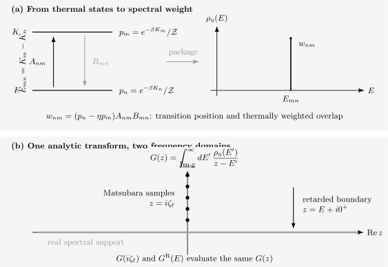
The Lehmann data separate transition energies, operator overlaps, and Gibbs populations. Their graded combination defines $\rho_\eta(E)$. A Cauchy transform of that measure produces both the discrete Matsubara values $G(i\zeta_n)$ and the retarded boundary $G(E+i0^+)$. The two frequency domains are evaluations of one analytic object, not independent fits.

Retarded Boundary Value

For the propagator convention,

$$\mathcal G_{AB}^{\mathrm R}(t) = - \frac{i}{\hbar} \theta(t) \left\langle [A(t),B(0)]_\eta \right\rangle_\beta.$$

Fourier transformation in energy gives

$$\mathcal G_{AB}^{\mathrm R}(E) = \int_{-\infty}^{\infty} dE'\, \frac{ \rho_{AB}^{(\eta)}(E') }{ E-E'+i0^+ }.$$

Similarly,

$$\mathcal G_{AB}^{\mathrm A}(E) = \int_{-\infty}^{\infty} dE'\, \frac{ \rho_{AB}^{(\eta)}(E') }{ E-E'-i0^+ }.$$

Using

$$\frac1{x+i0^+} = \operatorname{PV} \frac1x - i\pi\delta(x),$$

the discontinuity is

$$\mathcal G^{\mathrm R}(E) - \mathcal G^{\mathrm A}(E) = -2\pi i\, \rho^{(\eta)}(E).$$

Thus

$$\rho^{(\eta)}(E) = \frac{i}{2\pi} \left[ \mathcal G^{\mathrm R}(E) - \mathcal G^{\mathrm A}(E) \right].$$

For a scalar conjugate channel with the usual reality properties,

$$\rho^{(\eta)}(E) = - \frac1\pi \operatorname{Im} \mathcal G^{\mathrm R}(E).$$

The infinitesimal $i0^+$ selects causal support. It is not a linewidth. Replacing it by finite $\gamma$ is a separate physical, limiting, or numerical assumption.

Propagator and Observable Lanes

Two sign conventions recur often enough to deserve a direct dictionary.

Feature	Propagator lane	Observable-response lane
imaginary-time object	$\mathcal G=-\langle\mathcal T_\tau AB\rangle$	$C=+\langle\mathcal T_\tau\delta A\delta B\rangle$
real-time object	$\mathcal G^{\mathrm R}=-(i/\hbar)\theta\langle[A,B]_\eta\rangle$	$\chi^{\mathrm R}=+(i/\hbar)\theta\langle[\delta A,\delta B]\rangle$
Matsubara kernel	$\rho/(i\zeta-E)$	$\rho/(E-i\Omega)$
retarded kernel	$\rho/(E_{\rm ext}-E+i0^+)$	$\rho/(E-E_{\rm ext}-i0^+)$
common use	single-particle propagation	response to a classical source

For a bosonic observable channel with no static term,

$$C_{AB}(i\Omega_\ell) = \int_{-\infty}^{\infty} dE\, \frac{ \rho_{AB}^{(+)}(E) }{ E-i\Omega_\ell }.$$

Under the response source sign used elsewhere,

$$\chi_{AB}^{\mathrm R}(E_{\rm ext}) = \int_{-\infty}^{\infty} dE\, \frac{ \rho_{AB}^{(+)}(E) }{ E-E_{\rm ext}-i0^+ }.$$

These expressions are the same analytic function in the observable-response orientation. Since $C=-\mathcal G$ for the same bosonic operator pair, there is no physical contradiction.

A formula copied between the two columns without its defining sign will appear to disagree by a minus sign even when both sources are internally correct.

Bosonic Static Term

The most important qualification to the compact bosonic formula occurs at exactly zero transfer energy.

For connected bosonic observables, define the degenerate-transition weight

$$\begin{aligned} \Gamma_{AB} :={}& \sum_{\substack{n,m\\K_m=K_n}} p_n (\delta A)_{nm} (\delta B)_{mn}. \end{aligned}$$

These terms contribute a constant to the positive-sign Euclidean correlator:

$$C_{AB}^{\mathrm{static}}(\tau) = \Gamma_{AB}.$$

Its Matsubara transform is

$$C_{AB}^{\mathrm{static}}(i\Omega_\ell) = \beta\Gamma_{AB} \delta_{\ell0}.$$

But the bosonic commutator weight contains

$$p_n-p_m = 0$$

whenever $K_n=K_m$. The commutator spectral density therefore loses this exact static contribution.

Let $\rho_{AB,\mathrm{dyn}}^{(+)}$ denote the contribution from nondegenerate transitions. A complete observable representation is

$$\begin{aligned} C_{AB}(i\Omega_\ell) ={}& \int_{-\infty}^{\infty} dE\, \frac{ \rho_{AB,\mathrm{dyn}}^{(+)}(E) }{ E-i\Omega_\ell } \\ &+ \beta\Gamma_{AB} \delta_{\ell0}, \end{aligned}$$

The dynamic measure may have regular or continuum support through $E=0$. Only the exact degenerate contribution $\Gamma_{AB}$ is stored separately.

Connected does not mean dynamic

Subtracting

$$\delta A = A-\langle A\rangle$$

removes the disconnected product $\langle A\rangle\langle B\rangle$. It does not remove fluctuations inside a degenerate subspace or fluctuations of a conserved quantity.

If $Q$ commutes with $\mathcal K$, then

$$C_{QQ}(\tau) = \left\langle (\delta Q)^2 \right\rangle_\beta$$

is constant, while

$$\rho_{QQ}^{(+)}(E) = 0.$$

Consequently,

$$C_{QQ}(i\Omega_\ell) = \beta \operatorname{Var}_\beta(Q) \delta_{\ell0}.$$

The dynamic commutator response and the equilibrium static fluctuation answer different limiting questions. Discarding the Matsubara zero mode would erase the entire correlator in this example.

Why fermions differ

For a fermionic channel,

$$1+e^{-\beta E} \longrightarrow 2$$

as $E\to0$. A zero-energy fermionic transition is not annihilated by the graded anticommutator weight. The special missing-static-term mechanism is therefore bosonic.

High-Frequency Moments

For large $|z|$, formally write

$$\frac1{z-E} = \frac1z \sum_{r=0}^{\infty} \left( \frac{E}{z} \right)^r$$

and interpret the result as an asymptotic moment expansion when the required moments exist:

$$\frac1{z-E} = \frac1z + \frac{E}{z^2} + \frac{E^2}{z^3} + \cdots.$$

Then

$$\mathcal G_{AB}(z) \sim \frac{M_0}{z} + \frac{M_1}{z^2} + \frac{M_2}{z^3} + \cdots,$$

with

$$M_r := \int_{-\infty}^{\infty} dE\, E^r \rho_{AB}^{(\eta)}(E).$$

The first two moments are

$$M_0 = \left\langle [A,B]_\eta \right\rangle_\beta,$$

and

$$M_1 = \left\langle \left[ [A,\mathcal K], B \right]_\eta \right\rangle_\beta.$$

Higher moments contain further commutators with $\mathcal K$. They connect equal-time algebra to large-Matsubara-frequency tails.

For a canonical fermionic orbital,

$$M_0 = \left\langle \{c,c^\dagger\} \right\rangle = 1,$$

so

$$\mathcal G(i\nu_\ell) \sim \frac1{i\nu_\ell}$$

at large $|\nu_\ell|$. A computed tail with the wrong coefficient indicates missing spectral weight, a transform error, or a violated canonical algebra.

The full hierarchy of nested-commutator constraints belongs to Sum Rules.

Worked Benchmark: One Fermion Mode

Let

$$\mathcal K = \xi c^\dagger c.$$

The states $|0\rangle$ and $|1\rangle$ have

$$K_0=0, \qquad K_1=\xi,$$

and probabilities

$$p_0 = \frac1{1+e^{-\beta\xi}}, \qquad p_1 = \frac{e^{-\beta\xi}}{ 1+e^{-\beta\xi} }.$$

For $A=c$ and $B=c^\dagger$, the only nonzero matrix element connects $|1\rangle$ to $|0\rangle$. Therefore

$$\mathcal S^{>}(E) = p_0\delta(E-\xi),$$

and

$$\mathcal S^{<}(E) = p_1\delta(E-\xi).$$

The fermionic spectral density is

$$\begin{aligned} \rho^{(-)}(E) &= \left( p_0+p_1 \right) \delta(E-\xi) \\ &= \delta(E-\xi). \end{aligned}$$

The thermal probabilities cancel because $p_0+p_1=1$. The imaginary-time kernel restores the occupation dependence:

$$\mathcal G(\tau) = - \frac{ e^{-\xi\tau/\hbar} }{ 1+e^{-\beta\xi} }, \qquad 0\lt\tau\lt\beta\hbar.$$

Equivalently,

$$\mathcal G(\tau) = - \left[ 1-f(\xi) \right] e^{-\xi\tau/\hbar}.$$

The Matsubara and retarded functions are

$$\mathcal G(i\nu_\ell) = \frac1{ i\nu_\ell-\xi },$$

and

$$\mathcal G^{\mathrm R}(E) = \frac1{ E-\xi+i0^+ }.$$

The spectrum fixes the available orbital excitation; the Euclidean branch and lesser function encode how it is occupied.

Worked Benchmark: One Boson Mode

Let

$$\mathcal K = \epsilon b^\dagger b, \qquad \epsilon\gt0.$$

For $A=b$ and $B=b^\dagger$,

$$\mathcal S^{>}(E) = \left( 1+n_{\mathrm B}(\epsilon) \right) \delta(E-\epsilon),$$

while

$$\mathcal S^{<}(E) = n_{\mathrm B}(\epsilon) \delta(E-\epsilon).$$

Here

$$n_{\mathrm B}(\epsilon) = \frac1{ e^{\beta\epsilon}-1 }.$$

The bosonic commutator spectrum is

$$\rho^{(+)}(E) = \delta(E-\epsilon).$$

Again, the free-mode thermal factors cancel in the graded difference. The leading-minus propagator is

$$\mathcal D(\tau) = - \left( 1+n_{\mathrm B} \right) e^{-\epsilon\tau/\hbar},$$

for $0\lt\tau\lt\beta\hbar$, and

$$\mathcal D(i\Omega_\ell) = \frac1{ i\Omega_\ell-\epsilon }.$$

Its retarded boundary value is

$$\mathcal D^{\mathrm R}(E) = \frac1{ E-\epsilon+i0^+ }.$$

The stability condition $\epsilon\gt0$ is essential. At $\epsilon=0$, the grand-canonical occupation diverges and the one-mode Gibbs trace does not exist without further physics.

Worked Benchmark: Two-Level Observable

Consider

$$\mathcal K = \Delta|e\rangle\langle e|, \qquad \Delta\gt0,$$

with

$$A = |g\rangle\langle e| + |e\rangle\langle g|.$$

The Gibbs probabilities are

$$p_g = \frac1{ 1+e^{-\beta\Delta} }, \qquad p_e = \frac{ e^{-\beta\Delta} }{ 1+e^{-\beta\Delta} }.$$

The ordered spectrum is

$$\mathcal S^{>}_{AA}(E) = p_g\delta(E-\Delta) + p_e\delta(E+\Delta).$$

It obeys detailed balance because the negative-energy line has the smaller Boltzmann weight. The commutator spectral density is

$$\begin{aligned} \rho_{AA}^{(+)}(E) ={}& \left( p_g-p_e \right) \\ &\times \left[ \delta(E-\Delta) - \delta(E+\Delta) \right]. \end{aligned}$$

Since

$$p_g-p_e = \tanh \left( \frac{\beta\Delta}{2} \right),$$

the response weight vanishes at infinite temperature and approaches its ground-state value at low temperature.

Use the positive observable correlator

$$C_{AA}(\tau) = \left\langle \mathcal T_\tau A(\tau)A(0) \right\rangle.$$

For $0\lt\tau\lt\beta\hbar$,

$$C_{AA}(\tau) = p_g e^{-\Delta\tau/\hbar} + p_e e^{+\Delta\tau/\hbar}.$$

Its Matsubara transform is

$$C_{AA}(i\Omega_\ell) = \frac{ 2\Delta \tanh(\beta\Delta/2) }{ \Omega_\ell^2+\Delta^2 }.$$

At zero Matsubara frequency,

$$C_{AA}(0) = \frac{ 2 \tanh(\beta\Delta/2) }{ \Delta }.$$

This is a dynamic, nondegenerate example: no extra $\Gamma$ term is needed.

Chemical Potential and Energy Labels

When both the Gibbs state and time evolution use

$$\mathcal K = H-\mu\hat N,$$

the transfer energy is

$$E_{mn}^{(\mathcal K)} = \left( E_m^{(H)}-E_n^{(H)} \right) - \mu \left( N_m-N_n \right).$$

The KMS ratio is simply

$$\frac{p_m}{p_n} = e^{-\beta E_{mn}^{(\mathcal K)}}.$$

If operators evolve with $H$ instead, let

$$E_{mn}^{(H)} = E_m^{(H)}-E_n^{(H)},$$

and

$$\Delta N_{mn} = N_m-N_n.$$

Then

$$\frac{p_m}{p_n} = \exp \left[ -\beta \left( E_{mn}^{(H)} - \mu\Delta N_{mn} \right) \right].$$

For number-preserving observables, $\Delta N_{mn}=0$ and the two energy labels coincide. For particle addition or removal, the distinction shifts the spectral origin by chemical work. A spectral plot should state which generator defines zero energy.

Finite and Infinite Systems

For a finite closed system with a discrete spectrum,

$$\rho(E) = \sum_j w_j\delta(E-E_j).$$

The exact retarded function has distributional real-axis poles. Interactions can split and redistribute the residues, but they do not by themselves give exact finite-system eigenstates a decay width.

Smooth spectral weight can emerge through:

• a thermodynamic limit with dense levels;
• coupling to multiparticle continua;
• a genuinely open system;
• disorder or ensemble averaging;
• a declared numerical broadening;
• instrumental convolution.

These mechanisms are physically different. The spectral representation accommodates all of them through a measure, but it does not identify their origin automatically.

Numerical Evaluation

Exact diagonalization

For a finite basis:

1. diagonalize the same $\mathcal K$ used in the Gibbs state;
2. compute $E_{mn}$ and the relevant matrix elements;
3. exploit conserved quantum numbers to skip forbidden transitions;
4. accumulate $\mathcal S^>$ before forming graded differences;
5. keep exact zero-energy bosonic weight in a separate accumulator;
6. verify moments before applying any plotting kernel.

This ordering preserves positivity of the ordered spectrum and avoids subtracting nearly equal large numbers too early.

Stable thermal differences

For a bosonic transition,

$$p_n-p_m = p_n \left( 1-e^{-\beta E} \right).$$

When $|\beta E|\ll1$, evaluate

$$1-e^{-\beta E} = - \operatorname{expm1}(-\beta E)$$

numerically. Direct subtraction loses relative precision.

For fermionic weights $p_n+p_m$, use scaled exponentials or a log-sum-exp strategy when the spectrum spans many thermal decades.

Kernel evaluation

The bosonic factor

$$\frac{ \rho(E) }{ 1-e^{-\beta E} }$$

should be evaluated from a known regular limit near $E=0$, not by dividing two independently noisy arrays. An exact $\delta(E)$ term requires separate symbolic or discrete bookkeeping.

Broadening

Replacing

$$\delta(E-E_j)$$

with a Lorentzian or Gaussian may help visualization. Record the kernel, width, normalization, and whether moments are preserved. Never feed a broadened plot back into an exact sum rule without accounting for the tails and finite integration window.

Continuation boundary

Forward evaluation of $\mathcal G(\tau)$ or $\mathcal G(i\zeta_\ell)$ from a known spectrum is a well-conditioned integration problem. Recovering $\rho(E)$ from finitely many noisy values is an ill-posed inverse problem. Positivity, moments, symmetry, and causality constrain that inversion but do not manufacture resolution absent from the data. Analytic Continuation develops covariance whitening, singular-value diagnostics, regularization families, and feature-level evidence standards.

Physical Interpretation

Spectral support is operator resolved

A Hamiltonian eigenstate contributes only when the chosen operator pair has a nonzero matrix element. An absent line can reflect a selection rule rather than an absent state.

Thermal weights identify initial populations

The ordered spectrum uses $p_n$, because the system begins in $|n\rangle$. The reversed spectrum uses $p_m$. Their graded sum or difference determines which analytic Green function is being represented.

Imaginary-time decay is not real-time damping

A term

$$e^{-E\tau/\hbar}$$

reflects an energy difference in Euclidean time. It does not imply an irreversible lifetime. Real-time damping requires a continuum, an open-system mechanism, a limiting procedure, or another declared source of width.

Retardedness is boundary data

The spectral measure fixes where transitions occur. The $+i0^+$ prescription fixes how the analytic function approaches the real axis and therefore enforces causal support. Transition weight and temporal boundary condition are distinct pieces of information.

Static and dynamic information can separate

An exact bosonic zero mode can contribute to equilibrium fluctuations while disappearing from the commutator spectral density. Static thermodynamics, Matsubara zero modes, and real-time response must therefore be compared with their order of limits stated.

Validation Checklist

Before trusting a thermal spectral representation, check:

1. The same $\mathcal K$ defines the Gibbs state and the stated evolution, or the chemical-potential translation is explicit.
2. The operators have definite and correctly assigned parity.
3. The overall sign of the imaginary-time function is declared.
4. The energy-versus-angular-frequency convention is declared.
5. The ordered spectrum uses the initial-state weight $p_n$.
6. The reversed spectrum uses $p_m=e^{-\beta E}p_n$ on shell.
7. The graded density uses $p_n-\eta p_m$.
8. Matsubara frequencies satisfy $e^{i\beta\zeta_\ell}=\eta$.
9. Fermionic conjugate-channel spectral weight is nonnegative.
10. Bosonic negative-frequency commutator weight is not forced positive.
11. Exact bosonic zero-energy terms are stored separately.
12. The zeroth and available higher moments match equal-time algebra.
13. The high-frequency tail agrees with those moments.
14. A finite plotting width is not called an intrinsic lifetime.
15. Retarded data are obtained as boundary values of an analytic function, not by substituting into an arbitrary table.

Common Mistakes

• Calling every transition spectrum $\rho(E)$ without defining its operator order or bracket.
• Using $p_n-p_m$ for a fermionic anticommutator spectrum.
• Using $p_n+p_m$ for a bosonic commutator spectrum.
• Treating a bosonic commutator density as nonnegative at negative energy.
• Omitting the leading minus sign from one formula while retaining the propagator denominator convention from another.
• Combining an $H$-evolved spectrum with an $H-\mu N$ KMS factor.
• Concluding that temperature never changes a spectral density because it does not change a fixed Hamiltonian.
• Dividing by $1-e^{-\beta E}$ at $E=0$ without separating static weight.
• Assuming that subtracting $\langle A\rangle\langle B\rangle$ removes every zero mode.
• Interpreting Euclidean exponential decay as a quasiparticle lifetime.
• Replacing $i0^+$ by a finite number and calling the resulting width exact.
• Performing $i\zeta_\ell\to E+i0^+$ before identifying the analytic function and its asymptotics.

Reliable Workflow

1. Specify the ensemble and thermal generator.
2. Specify the operator pair, parity, and whether the channel changes particle number.
3. Declare the imaginary-time and real-time overall signs.
4. Insert a complete eigenbasis and define $E_{mn}$.
5. Build $\mathcal S^>(E)$ from $p_n$ and matrix elements.
6. Derive $\mathcal S^<(E)$ by KMS balance.
7. Form $\rho^{(\eta)}=\mathcal S^>-\eta\mathcal S^<$.
8. Isolate exact bosonic zero-energy weight.
9. Evaluate the desired Euclidean, Matsubara, or retarded transform.
10. Check moments, endpoints, symmetry, positivity where applicable, and asymptotic tails.
11. Apply broadening or numerical continuation only after the exact checks pass.

Cross-Links

• Matsubara Frequency Table – compact grid, units, parity, and transform normalization lookup.
• Finite-Temperature QM Overview – the common roadmap from Gibbs traces to imaginary time, Matsubara modes, spectra, and path integrals.
• Thermal Green Functions – ordering signs, contact jumps, equal-time limits, and free propagator benchmarks.
• Bosonic and Fermionic Matsubara Frequencies – frequency grids, units, index pairing, and zero-mode bookkeeping.
• Matsubara Formalism Preview – transforms, sums, convergence prescriptions, and diagrammatic use.
• Green Functions in Many-Body QM – particle addition and removal, fermionic positivity, occupations, and Dyson structure.
• Retarded and Advanced Response – causal support, boundary values, dispersion relations, and stability.
• Fluctuation–Dissipation Theorem – detailed balance, ordered and symmetrized spectra, and absorptive response.
• Spectral Functions – spectral line shapes, weights, widths, and measured intensities.
• Sum Rules – moment constraints and nested-commutator identities.
• Spectral Representation of Green Functions – resolvents and the spectral theorem.
• Correlation-Function Formula Sheet – compact convention and transform reference.

References

1. H. Lehmann, “On the Properties of Propagation Functions and Renormalization Constants of Quantized Fields”, Il Nuovo Cimento 11, 342–357 (1954).
2. T. Matsubara, “A New Approach to Quantum-Statistical Mechanics”, Progress of Theoretical Physics 14, 351–378 (1955).
3. R. Kubo, “Statistical-Mechanical Theory of Irreversible Processes. I”, Journal of the Physical Society of Japan 12, 570–586 (1957).
4. P. C. Martin and J. Schwinger, “Theory of Many-Particle Systems. I”, Physical Review 115, 1342–1373 (1959).
5. G. Baym and N. D. Mermin, “Determination of Thermodynamic Green’s Functions”, Journal of Mathematical Physics 2, 232–234 (1961).
6. A. L. Fetter and J. D. Walecka, Quantum Theory of Many-Particle Systems, Dover (2003 reprint of the 1971 edition), Chapters 3 and 7.
7. G. D. Mahan, Many-Particle Physics, 3rd ed., Springer (2000), Chapters 2 and 3.
8. J. W. Negele and H. Orland, Quantum Many-Particle Systems, Westview Press (1998), Chapters 2 and 3.
9. A. Altland and B. Simons, Condensed Matter Field Theory, 3rd ed., Cambridge University Press (2023), chapters on finite-temperature Green functions and linear response.
10. E. Gull, S. Iskakov, I. Krivenko, A. A. Rusakov, and D. Zgid, “Chebyshev Polynomial Representation of Imaginary-Time Response Functions”, Physical Review B 98, 075127 (2018).

Exercises

1. Derive the Matsubara denominator

Starting from

$$\mathcal G(\tau) = - \int dE\, e^{-E\tau/\hbar} \mathcal S^>(E),$$

derive the Matsubara representation for a channel satisfying

$$e^{i\beta\zeta_\ell} = \eta.$$

Identify the step at which the graded thermal weight appears.

Solution

Transform over one thermal interval:

$$\begin{aligned} \mathcal G(i\zeta_\ell) ={}& - \int dE\, \mathcal S^>(E) \\ &\times \frac1\hbar \int_0^{\beta\hbar} d\tau\, e^{(i\zeta_\ell-E)\tau/\hbar}. \end{aligned}$$

The integral is

$$\frac{ e^{\beta(i\zeta_\ell-E)}-1 }{ i\zeta_\ell-E }.$$

Using $e^{i\beta\zeta_\ell}=\eta$,

$$\begin{aligned} \mathcal G(i\zeta_\ell) &= \int dE\, \frac{ \left( 1-\eta e^{-\beta E} \right) \mathcal S^>(E) }{ i\zeta_\ell-E } \\ &= \int dE\, \frac{ \rho^{(\eta)}(E) }{ i\zeta_\ell-E }. \end{aligned}$$

The graded thermal factor enters when the endpoint exponential is replaced by the channel’s periodic or antiperiodic boundary phase.

2. Recover the free fermion branches

For

$$\rho^{(-)}(E) = \delta(E-\xi),$$

derive $\mathcal G(\tau)$ on $0\lt\tau\lt\beta\hbar$, its $0^+$ and $\beta\hbar^-$ limits, and $\mathcal G(i\nu_\ell)$.

Solution

The fermionic kernel gives

$$\mathcal G(\tau) = - \frac{ e^{-\xi\tau/\hbar} }{ 1+e^{-\beta\xi} }.$$

Since

$$1-f(\xi) = \frac1{ 1+e^{-\beta\xi} },$$

the positive-time branch is

$$\mathcal G(\tau) = - \left[ 1-f(\xi) \right] e^{-\xi\tau/\hbar}.$$

Therefore

$$\mathcal G(0^+) = - \left[ 1-f(\xi) \right],$$

and

$$\mathcal G(\beta\hbar^-) = -f(\xi).$$

Antiperiodicity identifies the latter with $-\mathcal G(0^-)$. Thus

$$\mathcal G(0^-) = f(\xi).$$

The spectral Cauchy transform gives

$$\mathcal G(i\nu_\ell) = \frac1{ i\nu_\ell-\xi }.$$

The contact jump is

$$\mathcal G(0^+) - \mathcal G(0^-) = -1.$$

3. Check two-level detailed balance

For the two-level observable in the worked example, compute

$$\frac{ \mathcal S^>(-\Delta) }{ \mathcal S^>(+\Delta) }$$

and show that the commutator spectrum is odd.

Solution

The two ordered weights are

$$\mathcal S^>(+\Delta) = p_g, \qquad \mathcal S^>(-\Delta) = p_e.$$

Their ratio is

$$\frac{p_e}{p_g} = e^{-\beta\Delta}.$$

This is detailed balance. The commutator density is

$$\begin{aligned} \rho^{(+)}(E) ={}& \left( p_g-p_e \right) \delta(E-\Delta) \\ &- \left( p_g-p_e \right) \delta(E+\Delta). \end{aligned}$$

Replacing $E$ by $-E$ exchanges the delta functions and contributes a minus sign:

$$\rho^{(+)}(-E) = -\rho^{(+)}(E).$$

4. Diagnose a conserved zero mode

Let $Q$ be Hermitian and satisfy

$$[Q,\mathcal K] = 0.$$

For $\delta Q=Q-\langle Q\rangle$, find the positive Euclidean correlator, its Matsubara transform, and its commutator spectral density.

Solution

Conservation gives

$$\delta Q(\tau) = \delta Q.$$

Therefore

$$C_{QQ}(\tau) = \left\langle (\delta Q)^2 \right\rangle_\beta = \operatorname{Var}_\beta(Q).$$

The transform of a constant is

$$\begin{aligned} C_{QQ}(i\Omega_\ell) &= \frac{ \operatorname{Var}_\beta(Q) }{\hbar} \int_0^{\beta\hbar} d\tau\, e^{i\Omega_\ell\tau/\hbar} \\ &= \beta \operatorname{Var}_\beta(Q) \delta_{\ell0}. \end{aligned}$$

Because the commutator vanishes,

$$\rho_{QQ}^{(+)}(E) = 0.$$

The entire correlator is a static bosonic Matsubara zero mode. It cannot be reconstructed from the commutator spectrum alone.

5. Obtain the first two moments

Use the Lehmann definition of $\rho^{(\eta)}$ to prove

$$M_0 = \langle[A,B]_\eta\rangle_\beta,$$

and

$$M_1 = \left\langle \left[ [A,\mathcal K], B \right]_\eta \right\rangle_\beta.$$

Solution

Integrating the zeroth moment removes the delta function:

$$M_0 = \sum_{n,m} \left( p_n-\eta p_m \right) A_{nm}B_{mn}.$$

The first term is $\langle AB\rangle$. Relabeling $n\leftrightarrow m$ in the second term gives $\langle BA\rangle$. Hence

$$M_0 = \langle AB-\eta BA\rangle = \langle[A,B]_\eta\rangle.$$

For the first moment, use

$$\left( [A,\mathcal K] \right)_{nm} = \left( K_m-K_n \right) A_{nm}.$$

The same relabeling then yields

$$M_1 = \left\langle [A,\mathcal K]B - \eta B[A,\mathcal K] \right\rangle,$$

which is

$$M_1 = \left\langle \left[ [A,\mathcal K], B \right]_\eta \right\rangle.$$

6. Translate the chemical-potential convention

Suppose

$$[H,\hat N]=0$$

and an operator changes particle number by $q$:

$$[\hat N,A] = -qA.$$

Relate its $H$-evolved and $\mathcal K=H-\mu\hat N$-evolved forms, and state the corresponding shift of spectral energy.

Solution

Since $H$ and $\hat N$ commute,

$$\begin{aligned} A_{\mathcal K}(t) ={}& e^{i(H-\mu\hat N)t/\hbar} A \\ &\times e^{-i(H-\mu\hat N)t/\hbar} \\ ={}& e^{iHt/\hbar} e^{-i\mu\hat Nt/\hbar} A \\ &\times e^{i\mu\hat Nt/\hbar} e^{-iHt/\hbar}. \end{aligned}$$

The number commutator gives

$$e^{-i\mu\hat Nt/\hbar} A e^{i\mu\hat Nt/\hbar} = e^{iq\mu t/\hbar}A.$$

Therefore

$$A_{\mathcal K}(t) = e^{iq\mu t/\hbar} A_H(t).$$

The energy-domain transform is shifted by

$$E_{\mathcal K} = E_H-q\mu.$$

Equivalently, a transition changing particle number by $\Delta N=q$ has

$$\Delta K = \Delta H-\mu q.$$

7. Prove the channel-dependent sign constraint

Assume $B=A^\dagger$. Show that the fermionic graded spectral density is nonnegative, while a bosonic commutator density satisfies

$$E\rho^{(+)}(E) \geq 0$$

for each diagonal transition in a Gibbs state.

Solution

For a conjugate channel,

$$A_{nm}B_{mn} = |A_{nm}|^2 \geq 0.$$

In a fermionic channel the coefficient is

$$p_n+p_m \geq 0.$$

Every Lehmann line is therefore nonnegative.

In a bosonic channel,

$$p_n-p_m = p_n \left( 1-e^{-\beta E} \right)$$

on a line at $E=K_m-K_n$. The factor $1-e^{-\beta E}$ has the same sign as $E$. Thus

$$E \left( p_n-p_m \right) |A_{nm}|^2 \geq 0$$

term by term. Summing all transitions gives the stated distributional sign constraint. The density itself is negative at negative energy, so ordinary nonnegativity would be the wrong test.