Finite-Temperature QM Overview

Finite-temperature quantum mechanics is the equilibrium framework in which a Gibbs operator supplies statistical weights, imaginary time organizes operator products, and thermal correlation functions connect thermodynamics to spectra and response.

The central structural identity is

$$e^{-\beta\mathcal K} = e^{-\mathcal K(\beta\hbar)/\hbar}.$$

Here $\beta=(k_{\mathrm B}T)^{-1}$ and $\mathcal K$ is the generator appropriate to the ensemble. For a canonical ensemble,

$$\mathcal K=H,$$

whereas for a grand-canonical ensemble with a conserved particle number,

$$\mathcal K=H-\mu N, \qquad [H,N]=0.$$

The Gibbs weight therefore has the algebraic form of evolution through an imaginary-time interval of length $\beta\hbar$. Taking a trace closes that interval into a thermal circle. This observation leads to imaginary-time ordering, the Kubo–Martin–Schwinger relation, bosonic and fermionic boundary conditions, discrete Matsubara frequencies, equilibrium path integrals, and a controlled bridge to real-frequency response.

The resemblance to time evolution is powerful but must be interpreted correctly. Imaginary time is a calculational coordinate for equilibrium quantum statistics. It is not laboratory time, and evolution by $e^{-\tau\mathcal K/\hbar}$ is not unitary dynamics.

Purpose and Canonical Scope

This page is a map of the finite-temperature toolkit. It develops the common operator structure far enough to show why the methods fit together and how to choose among them.

Several nearby pages own the detailed ingredients:

• Thermal Density Operators owns the Gibbs state, its normalization, entropy, temperature limits, and domain of validity.
• Partition Functions owns derivatives of $Z$, thermodynamic potentials, and fluctuation identities.
• Finite-Temperature Phase Transitions owns thermal nonanalyticity, transition order, critical temperatures, critical fluctuations, and finite-size rounding.
• Time-Dependent Correlations owns the general real-time correlation dictionary.
• Green Functions in Many-Body QM owns particle-addition and particle-removal propagators, their Lehmann representation, and the normal-state spectral convention.
• Spectral Functions owns line shapes, poles, continua, sum rules, and the relation between spectra and experiments.
• Euclidean and Imaginary-Time Path Integrals owns Wick rotation, open Euclidean kernels, elementary time slicing, and projection.
• Path Integrals for Statistical Mechanics owns the closed thermal trace, cyclic measure, exchange sectors, ring-polymer mapping, and oscillator determinant.
• Coherent-State Path Integrals Preview owns bosonic and fermionic coherent-state traces, Grassmann integration, determinant rules, and symbol-ordering cautions.
• Diagrammatic Methods Preview fixes a concrete many-body diagram convention and explains how Matsubara graphs differ from Goldstone and real-time graphs.
• Bosonic and Fermionic Matsubara Frequencies owns the frequency grids, explicit-$\hbar$ units, index pairing, zero modes, and finite-cutoff conventions.
• Thermal Green Functions owns graded two-point definitions, one-sided equal-time limits, contact terms, and free fermion and boson benchmarks.
• Spectral Representation owns thermal Lehmann weights, Euclidean kernels, Matsubara Cauchy transforms, retarded boundary values, and static bosonic terms.
• Analytic Continuation owns finite-data inversion, covariance, regularization families, resolution tests, and reporting standards.

Imaginary Time develops the operator semigroup, heat-equation form, open-versus-closed boundaries, and projection role. Matsubara Formalism Preview develops the compact-time Fourier workflow, loop sums, convergence prescriptions, and QFT handoff. Finite-Temperature QFT Bridge carries that handoff to thermal field propagators, vacuum-versus-thermal loop terms, screening, zero-mode effective theory, and real-time boundaries. Path Integrals for Statistical Mechanics gives the regulated coordinate construction, while Coherent-State Path Integrals Preview gives the Fock-space construction. The remaining pages specialize the roadmap into KMS structure and real-time thermal dynamics.

Prerequisites and Working Conventions

The minimum prerequisites are:

1. density operators and trace expectation values;
2. canonical and grand-canonical ensembles;
3. Heisenberg-picture operator evolution;
4. creation and annihilation operators;
5. basic Fourier-series reasoning.

This chapter keeps $\hbar$ explicit. Imaginary time $\tau$ has dimensions of time and lies on

$$0 \leq \tau \lt \beta\hbar.$$

Many texts instead use a variable with dimensions of inverse energy and write $0\leq\tau\lt\beta$. The two conventions differ by a factor of $\hbar$. A formula should never mix them silently.

We use:

Symbol	Meaning	Units
$\beta$	inverse temperature $(k_{\mathrm B}T)^{-1}$	inverse energy
$\mathcal K$	ensemble generator	energy
$\tau$	imaginary time	time
$\omega_n$	angular Matsubara frequency	inverse time
$\nu_n=\hbar\omega_n$	Matsubara energy	energy
$\mathcal T_\tau$	imaginary-time ordering	none

For a canonical calculation, replace $\mathcal K$ by $H$. For a grand-canonical calculation, using $\mathcal K=H-\mu N$ consistently is essential: it is the source of the familiar one-particle energy

$$\xi_{\mathbf k} = \epsilon_{\mathbf k}-\mu.$$

From Gibbs Weight to Imaginary Time

Real-time evolution generated by a time-independent Hamiltonian is

$$U(t) = e^{-iHt/\hbar}.$$

Formally substituting $t=-i\tau$ gives

$$U(-i\tau) = e^{-H\tau/\hbar}.$$

At the thermal interval $\tau=\beta\hbar$,

$$U(-i\beta\hbar) = e^{-\beta H}.$$

This is the unnormalized canonical Gibbs operator. More generally,

$$\rho_{\beta} = \frac{e^{-\beta\mathcal K}}{\mathcal Z}, \qquad \mathcal Z = \operatorname{Tr}e^{-\beta\mathcal K}.$$

Spectral meaning

Let

$$\mathcal K|n\rangle = \kappa_n|n\rangle.$$

Then

$$e^{-\tau\mathcal K/\hbar}|n\rangle = e^{-\tau\kappa_n/\hbar}|n\rangle.$$

Imaginary-time evolution exponentially suppresses larger $\kappa_n$ relative to smaller $\kappa_n$. It is therefore nonunitary. In particular,

$$\left( e^{-\tau\mathcal K/\hbar} \right)^\dagger e^{-\tau\mathcal K/\hbar} = e^{-2\tau\mathcal K/\hbar},$$

which is not generally the identity.

The same suppression explains both thermal weighting and ground-state projection:

• setting $\tau=\beta\hbar$ produces Boltzmann weights;
• taking a long open interval $\tau\to\infty$ projects a trial state toward its lowest-$\mathcal K$ component, when that component is present and the spectrum is bounded below.

Thermal traces and ground-state projection use the same semigroup, but their boundary conditions and physical questions differ.

Thermal averages

For an observable $A$,

$$\langle A\rangle_{\beta} = \frac{ \operatorname{Tr} \left( e^{-\beta\mathcal K}A \right) }{ \mathcal Z }.$$

If $A$ commutes with $\mathcal K$, the expectation is an ordinary Boltzmann-weighted spectral average. When $A$ does not commute with $\mathcal K$, imaginary-time dependence preserves the noncommuting operator structure rather than reducing the problem to classical probabilities.

Why the Trace Creates a Thermal Circle

For a particle with coordinate basis $|q\rangle$,

$$Z = \int dq\, \langle q| e^{-\beta H} |q\rangle.$$

The same coordinate appears at both ends because of the trace. After inserting many resolutions of the identity, the matrix element becomes a sum over paths with

$$q(\beta\hbar) = q(0).$$

The imaginary-time interval is therefore compact: its endpoints are identified.

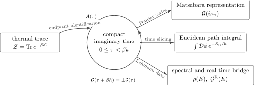
The thermal trace turns $e^{-\beta\mathcal K}$ into propagation around a compact imaginary-time direction. Operator ordering, Fourier modes, path integrals, and spectral reconstruction are different representations of this same equilibrium structure.

The circle is not an extra spatial dimension in the original quantum system. It is a representation of the thermal trace. In field theory the same construction becomes a Euclidean spacetime with compact imaginary time, but additional issues such as renormalization, gauge symmetry, and Lorentzian reconstruction belong to the field-theory treatment.

Imaginary-Time Operators

Define

$$A(\tau) = e^{\tau\mathcal K/\hbar} A e^{-\tau\mathcal K/\hbar}.$$

Differentiation gives the imaginary-time Heisenberg equation

$$\hbar \frac{\partial A(\tau)}{\partial\tau} = \left[ \mathcal K,A(\tau) \right].$$

Compare this with real time:

$$i\hbar \frac{\partial A(t)}{\partial t} = \left[ A(t),H \right].$$

The missing factor of $i$ is responsible for exponential rather than oscillatory behavior.

For two operators, define the unordered imaginary-time correlator

$$C_{AB}(\tau) = \left\langle A(\tau)B(0) \right\rangle_{\beta}.$$

In an eigenbasis of $\mathcal K$,

$$\begin{aligned} C_{AB}(\tau) &= \frac1{\mathcal Z} \sum_{m,n} e^{-\beta\kappa_m} e^{\tau(\kappa_m-\kappa_n)/\hbar} \\ &\quad\times \langle m|A|n\rangle \langle n|B|m\rangle. \end{aligned}$$

This formula already contains the main finite-temperature ingredients:

• thermal weights $e^{-\beta\kappa_m}$;
• excitation-energy differences $\kappa_n-\kappa_m$;
• matrix elements selecting the observable channel;
• exponential decay or growth along the finite imaginary-time interval.

The finite interval and KMS relation prevent the apparent growth terms from causing an inconsistency.

KMS Cyclicity

The trace identity behind equilibrium periodicity is especially important. Since

$$A(\tau+\beta\hbar) = e^{\beta\mathcal K} A(\tau) e^{-\beta\mathcal K},$$

one obtains

$$\begin{aligned} \left\langle A(\tau+\beta\hbar)B \right\rangle_{\beta} &= \frac1{\mathcal Z} \operatorname{Tr} \left[ A(\tau)e^{-\beta\mathcal K}B \right] \\ &= \left\langle BA(\tau) \right\rangle_{\beta}. \end{aligned}$$

This is an imaginary-time form of the Kubo–Martin–Schwinger condition. It exchanges the operator order when one insertion is moved once around the thermal circle.

Two distinctions matter:

1. the trace identity itself does not insert a fermionic minus sign;
2. antiperiodicity of a fermionic Green function arises when KMS cyclicity is combined with graded imaginary-time ordering.

Confusing these steps is a common source of sign errors.

Imaginary-Time Ordering

For operators of definite fermion parity, define

$$\eta = \begin{cases} +1, & \text{bosonic or even operators},\\ -1, & \text{fermionic or odd operators}. \end{cases}$$

For two operators of the same parity,

$$\begin{aligned} \mathcal T_\tau A(\tau)B(\tau') &= \theta(\tau-\tau') A(\tau)B(\tau') \\ &\quad+ \eta\, \theta(\tau'-\tau) B(\tau')A(\tau). \end{aligned}$$

The sign $\eta=-1$ records one exchange of odd operators. A common Green-function convention is

$$\mathcal G_{AB}(\tau-\tau') = - \left\langle \mathcal T_\tau A(\tau)B(\tau') \right\rangle_{\beta}.$$

The overall minus sign is conventional and must be checked for each channel. Response functions, coordinate correlators, spin correlators, and single-particle propagators do not all use identical prefactors.

KMS cyclicity and graded ordering imply

$$\mathcal G_{AB} (\tau+\beta\hbar) = \eta\, \mathcal G_{AB}(\tau).$$

Thus:

$$\begin{aligned} \mathcal G_{\mathrm B} (\tau+\beta\hbar) &= \mathcal G_{\mathrm B}(\tau), \\ \mathcal G_{\mathrm F} (\tau+\beta\hbar) &= - \mathcal G_{\mathrm F}(\tau). \end{aligned}$$

Composite operators inherit the parity of the full operator. A fermion density $\psi^\dagger\psi$ is even and therefore has bosonic thermal boundary conditions, despite being built from fermionic fields.

Matsubara Frequencies

A function on a compact interval has a Fourier series. Periodicity or antiperiodicity quantizes its allowed frequencies.

Bosonic modes

For

$$F(\tau+\beta\hbar) = F(\tau),$$

the angular Matsubara frequencies are

$$\omega_n^{\mathrm B} = \frac{ 2\pi n }{ \beta\hbar }, \qquad n\in\mathbb Z.$$

Fermionic modes

For

$$F(\tau+\beta\hbar) = -F(\tau),$$

the angular Matsubara frequencies are

$$\omega_n^{\mathrm F} = \frac{ (2n+1)\pi }{ \beta\hbar }, \qquad n\in\mathbb Z.$$

In energy units,

$$\nu_n = \hbar\omega_n,$$

so that

$$\begin{aligned} \nu_n^{\mathrm B} &= \frac{2\pi n}{\beta}, \\ \nu_n^{\mathrm F} &= \frac{(2n+1)\pi}{\beta}. \end{aligned}$$

The bosonic spectrum contains a zero mode at $n=0$. The fermionic spectrum does not. This difference has major consequences for long-distance finite-temperature physics.

Fourier pair

Using Matsubara energies, a convenient convention is

$$\mathcal G(i\nu_n) = \frac1\hbar \int_0^{\beta\hbar} d\tau\, e^{i\nu_n\tau/\hbar} \mathcal G(\tau),$$

with inverse

$$\mathcal G(\tau) = \frac1\beta \sum_n e^{-i\nu_n\tau/\hbar} \mathcal G(i\nu_n).$$

The sum runs over the bosonic or fermionic sequence appropriate to the operator channel. In conventions where $\hbar=k_{\mathrm B}=1$, the distinction among $\tau$, $\beta$, angular frequency, and energy is hidden. Restoring units after a calculation requires knowing which convention was used.

Five Equivalent Windows on Equilibrium

Finite-temperature calculations repeatedly move among five representations.

Representation	Basic object	Especially useful for	Main caution
operator trace	$\operatorname{Tr}(e^{-\beta\mathcal K}\cdots)$	exact identities, symmetries, finite spectra	Hilbert-space dimension grows rapidly
imaginary time	$\mathcal G(\tau)$	equilibrium ordering and decay	$\tau$ is not real time
Matsubara frequency	$\mathcal G(i\nu_n)$	convolutions, diagrams, frequency sums	frequencies are discrete and imaginary
spectral form	$\rho(E)$ or $A(E)$	excitations, sum rules, real-frequency bridge	normalization and signs are channel dependent
Euclidean path integral	$\int\mathcal D\phi\,e^{-S_{\mathrm E}/\hbar}$	collective fields, saddle points, Monte Carlo	measure, discretization, and sign problems matter

These are not five different theories. Under their assumptions, they are reorganizations of the same equilibrium trace.

Spectral Representation and Real-Frequency Bridge

The eigenstate sum shows that imaginary-time correlators are built from transition energies. A spectral density packages those transitions into a function of real energy.

For many standard channels, one can define an analytic function of a complex energy $z$,

$$\mathcal G(z) = \int_{-\infty}^{\infty} dE\, \frac{ \rho(E) }{ z-E }.$$

The detailed definition of $\rho(E)$ depends on the operator, bracket, and normalization. Once those conventions are fixed, Matsubara data sample

$$z=i\nu_n,$$

whereas the retarded function is the boundary value at

$$z=E+i0^+.$$

This motivates the formal continuation

$$i\nu_n \longrightarrow E+i0^+.$$

The arrow is shorthand for evaluating the same analytic function at a different boundary. It is not a substitution rule for an arbitrary finite table of Matsubara values.

Imaginary time is a smoothed spectral transform

For the normal fermionic single-particle convention used in Green Functions in Many-Body QM, one has for $0\lt\tau\lt\beta\hbar$

$$\mathcal G(\tau) = - \int_{-\infty}^{\infty} dE\, \frac{ e^{-E\tau/\hbar} }{ 1+e^{-\beta E} } A(E).$$

The kernel smooths the spectral function. Narrow peaks and nearby thresholds can produce very similar imaginary-time data, especially after statistical noise and finite sampling are included.

Exact Matsubara values at all frequencies, together with appropriate analyticity and asymptotic information, can determine the real-frequency function in principle. Numerical continuation from finitely many noisy values is ill posed. Analytic Continuation develops this inverse problem in detail. A credible reconstruction therefore reports:

• the assumed spectral class and positivity properties;
• sum rules and high-frequency moments;
• uncertainty propagation;
• sensitivity to priors or regularization;
• synthetic-data resolution tests;
• stability under removing data points;
• which claimed features are actually resolved.

Spectral Representation derives the exact thermal bridge and its channel-dependent signs. Spectral Functions owns the evidence standard for reconstructed line shapes. Retarded and Advanced Response owns causal response conventions.

Equilibrium Path Integrals

The operator exponential can be divided into $M$ short factors:

$$e^{-\beta H} = \left( e^{-\Delta\tau H/\hbar} \right)^M, \qquad \Delta\tau = \frac{\beta\hbar}{M}.$$

Inserting complete sets between the factors and taking $M\to\infty$ gives, for a particle with

$$H = \frac{p^2}{2m} +V(q),$$

the formal Euclidean path integral

$$Z = \int_{q(\beta\hbar)=q(0)} \mathcal Dq\, e^{-S_{\mathrm E}[q]/\hbar},$$

where

$$S_{\mathrm E}[q] = \int_0^{\beta\hbar} d\tau\, \left[ \frac{m}{2} \left( \frac{dq}{d\tau} \right)^2 +V(q) \right].$$

The oscillatory real-time weight $e^{iS/\hbar}$ has become the decaying Euclidean weight $e^{-S_{\mathrm E}/\hbar}$. This often makes equilibrium path integrals suitable for saddle-point expansions and stochastic sampling.

Several qualifications are essential:

• the trace enforces a closed imaginary-time boundary condition;
• a time-sliced definition is needed before the continuum notation is meaningful;
• operator ordering can generate discretization corrections;
• first-quantized identical-particle traces include permutation sectors;
• bosonic coherent-state fields are periodic;
• fermionic coherent-state fields are Grassmann-valued and antiperiodic;
• a Euclidean weight need not be real and nonnegative, so Monte Carlo can face a sign or phase problem.

The path integral is a representation, not an approximation. Approximations enter through discretization, saddle-point truncation, perturbative expansion, variational ansatz, or numerical sampling.

Worked Example: A Two-Level Thermal Correlator

Consider

$$H = \frac{\Delta}{2}\sigma_z, \qquad \Delta>0,$$

with

$$Z = 2\cosh \left( \frac{\beta\Delta}{2} \right).$$

Take $A=B=\sigma_x$. Since $\sigma_x$ connects the two energy eigenstates, the eigenbasis formula gives, for $0\leq\tau\leq\beta\hbar$,

$$\begin{aligned} C_{xx}(\tau) &= \left\langle \sigma_x(\tau)\sigma_x(0) \right\rangle_\beta \\ &= \frac{ e^{\beta\Delta/2} e^{-\Delta\tau/\hbar} +e^{-\beta\Delta/2} e^{\Delta\tau/\hbar} }{ 2\cosh(\beta\Delta/2) }. \end{aligned}$$

Equivalently,

$$C_{xx}(\tau) = \frac{ \cosh \left[ \Delta \left( \frac{\beta}{2} -\frac{\tau}{\hbar} \right) \right] }{ \cosh(\beta\Delta/2) }.$$

This compact expression makes several checks immediate:

$$\begin{aligned} C_{xx}(0) &= 1, \\ C_{xx}(\beta\hbar) &= 1, \\ C_{xx}(\beta\hbar-\tau) &= C_{xx}(\tau). \end{aligned}$$

Because $\sigma_x$ is an even observable in this spin problem, the thermal correlator is bosonic. Its Matsubara energies are $\nu_n=2\pi n/\beta$. The transform is

$$C_{xx}(i\nu_n) = \frac{ 2\Delta \tanh(\beta\Delta/2) }{ \Delta^2+\nu_n^2 }.$$

At low temperature and fixed positive $\tau$,

$$C_{xx}(\tau) \longrightarrow e^{-\Delta\tau/\hbar}.$$

The imaginary-time decay rate directly reveals the excitation gap $\Delta$. At finite temperature, propagation can begin from either thermally occupied level, producing the two exponentials in the exact result.

Worked Benchmark: One Fermionic Mode

For

$$\mathcal K = \xi c^\dagger c, \qquad \xi = \epsilon-\mu,$$

the Fermi occupation is

$$f(\xi) = \frac1{ e^{\beta\xi}+1 }.$$

For $0<\tau<\beta\hbar$, the exact branch is

$$\mathcal G(\tau) = - \left[ 1-f(\xi) \right] e^{-\xi\tau/\hbar}.$$

For $-\beta\hbar<\tau<0$,

$$\mathcal G(\tau) = f(\xi) e^{-\xi\tau/\hbar}.$$

They glue antiperiodically and transform to

$$\mathcal G(i\nu_n) = \frac1{ i\nu_n-\xi }.$$

Thermal Green Functions owns the derivation, one-sided equal-time limits, contact jump, free boson comparison, and physical interpretation. This overview retains the result only as a compact method benchmark.

Choosing a Finite-Temperature Method

The observable and desired output should determine the representation.

Question	Natural starting object	Typical method
free energy or equation of state	$\mathcal Z$ or $\ln\mathcal Z$	exact spectrum, linked expansion, path integral
equal-time expectation	$\operatorname{Tr}(\rho_\beta A)$	operator algebra, diagonalization, Monte Carlo estimator
static susceptibility	equilibrium covariance or zero-frequency response	derivatives of $\ln\mathcal Z$, Kubo formula
excitation spectrum	real-frequency spectral function	Lehmann representation, analytic continuation, real-time method
perturbative equilibrium correction	Matsubara Green functions	frequency sums and diagrams
strongly coupled equilibrium observable	Euclidean path integral or tensor-network thermal state	Monte Carlo, purification, typicality, specialized solver
transient or driven dynamics	contour-ordered real-time correlator	Keldysh or other nonequilibrium method

No representation is universally superior. Exact diagonalization is transparent but size limited. Matsubara perturbation theory is systematic near a controlled reference but can fail at strong coupling or near infrared singularities. Euclidean Monte Carlo can be nonperturbative but may suffer finite-size, discretization, autocorrelation, and sign problems. Analytic continuation may dominate the uncertainty even when imaginary-time data are precise.

A Reliable Calculation Workflow

1. State the ensemble

Specify

$$\rho = \frac{e^{-\beta\mathcal K}}{\mathcal Z}$$

and define every chemical potential and conserved charge in $\mathcal K$.

2. Check that the trace exists

For a finite system, verify that $e^{-\beta\mathcal K}$ is trace class. In continuum or infinite-volume problems, introduce the physical volume, regulator, or thermodynamic-limit prescription before manipulating $Z$.

3. Identify operator parity and channel

Decide whether the correlator is:

• bosonic or fermionic under thermal boundary conditions;
• number preserving or number changing;
• ordered, symmetrized, retarded, advanced, lesser, or greater;
• scalar, matrix-valued, or carrying momentum and internal indices.

4. Fix transform conventions

State whether the frequency variable is $\omega_n$ or $\nu_n=\hbar\omega_n$, and record all factors of $\beta$, $\hbar$, and volume.

5. Compute in the representation suited to the problem

Use spectral sums for small systems, Matsubara diagrams for controlled perturbation theory, path integrals for collective or stochastic formulations, and real-time methods for explicitly dynamical questions.

6. Enforce exact checks

Useful checks include:

• KMS periodicity or antiperiodicity;
• equal-time commutator or anticommutator jumps;
• spectral normalization;
• high-frequency moments;
• Hermiticity and positivity constraints;
• conservation-law Ward identities;
• thermodynamic derivative identities.

7. Separate exact transformations from inference

An exact Fourier series from $\tau$ to $i\nu_n$ is not the same task as inferring a real-frequency spectrum from noisy data. Report analytic-continuation assumptions as part of the result.

8. Audit physical limits

Check low and high temperature, weak and strong coupling where known, finite-size scaling, and the order of zero-frequency and zero-momentum limits.

Temperature and Scale Hierarchies

Temperature introduces the energy scale

$$k_{\mathrm B}T = \frac1\beta.$$

Its significance depends on comparison with gaps, bandwidths, interaction energies, finite-size spacings, and probe frequencies.

Low temperature

If a finite system has a unique ground state and gap $\Delta$, then thermal corrections to many equilibrium quantities are suppressed by

$$e^{-\beta\Delta}.$$

The thermal circle becomes long:

$$\beta\hbar \to \infty.$$

Imaginary-time correlators can then display a broad window of ground-state exponential decay. Degenerate ground spaces, gapless systems, and thermodynamic limits require more care.

High temperature

As $\beta\to0^+$, the thermal circle shrinks. A high-temperature expansion organizes powers of $\beta H$ only when the relevant operator products and traces are controlled. In an infinite-dimensional Hilbert space, the formal state proportional to the identity may not be normalizable.

Matsubara spacing

Adjacent bosonic Matsubara energies differ by

$$\Delta\nu = \frac{2\pi}{\beta} = 2\pi k_{\mathrm B}T.$$

At lower temperature the grid becomes denser and approaches a continuum. At higher temperature nonzero modes are widely separated, but the bosonic zero mode remains. Long-distance thermal behavior can therefore be dominated by static bosonic fluctuations.

Finite size versus temperature

Let $\delta_L$ be a characteristic finite-size level spacing. Then:

• $k_{\mathrm B}T\ll\delta_L$ resolves individual low-lying levels;
• $k_{\mathrm B}T\gg\delta_L$ thermally averages over many levels;
• taking $L\to\infty$ before $T\to0$ can differ from reversing the limits.

The order of limits is part of the physical statement, especially near phase transitions and in systems with conserved quantities.

What the Formalism Does Not Assume

Finite-temperature equilibrium methods do not by themselves assume:

• weak interactions;
• nondegenerate perturbation theory;
• quasiparticles;
• a classical limit;
• a continuum;
• the thermodynamic limit;
• that an isolated system dynamically thermalizes;
• that Euclidean data can be continued stably to real time.

They do assume that an equilibrium state and its generator have been specified. Whether a physical preparation reaches that state is a separate dynamical question.

Equilibrium Versus Nonequilibrium

The thermal circle encodes a stationary Gibbs ensemble. It is well suited to:

• thermodynamics;
• equilibrium correlations;
• static response;
• imaginary-frequency perturbation theory;
• equilibrium spectral constraints.

It is not sufficient for a general quench, drive, transient, or current-carrying steady state. Nonequilibrium calculations typically require an initial density operator plus forward and backward real-time evolution. Retarded response near equilibrium can be obtained from equilibrium correlations, but nonlinear and far-from-equilibrium dynamics require additional information.

The Kubo Formula owns the linear-response derivation. Transport Coefficients Preview owns the equilibrium-to-hydrodynamic transport dictionary. Full closed-time-path field theory belongs to the later QFT bridge.

Common Mistakes

• Treating imaginary time as physical time. The map $t=-i\tau$ reorganizes equilibrium amplitudes; $e^{-\tau H/\hbar}$ is nonunitary.
• Using $H$ where the grand-canonical generator is required. A charged field evolves with $\mathcal K=H-\mu N$, which produces energies relative to $\mu$.
• Dropping $\hbar$ inconsistently. If $\tau$ has units of time, the interval is $\beta\hbar$, not $\beta$.
• Assigning boundary conditions from constituent fields. A density made from fermions is even and has bosonic Matsubara frequencies.
• Putting a fermionic minus sign into trace cyclicity. The sign arises from graded ordering, not from the ordinary trace.
• Assuming every thermal correlator uses the same leading minus sign. Definitions differ among propagators, susceptibilities, and structure factors.
• Forgetting the equal-time jump. Fermionic Green functions are antiperiodic but discontinuous at coincident time because of the canonical anticommutator.
• Confusing Matsubara and retarded functions. They are values or boundary limits of an analytic object in different domains.
• Continuing individual discrete values by substitution. Analytic continuation acts on a justified analytic representation after sums and algebra are complete.
• Reading numerical continuation as unique. Finite noisy imaginary-time data generally support a family of compatible spectra.
• Calling a Euclidean path integral automatically positive. Fermion determinants, chemical potentials, frustration, and topological terms can generate sign or phase problems.
• Equating a Gibbs state with a thermalization mechanism. Equilibrium state definition and dynamical approach to equilibrium are distinct questions.
• Ignoring finite volume. Traces, zero modes, singularities, and phase transitions can change qualitatively in the thermodynamic limit.
• Reversing limits without comment. Static, uniform, zero-temperature, and infinite-volume limits may not commute.

Compact Method Dictionary

If you see	Read it as
$e^{-\beta\mathcal K}$	unnormalized equilibrium weight
$\tau\in[0,\beta\hbar)$	compact imaginary-time coordinate
$\mathcal T_\tau$	graded ordering along the thermal circle
$2\pi n/\beta$	bosonic Matsubara energy
$(2n+1)\pi/\beta$	fermionic Matsubara energy
$i\nu_n$	discrete imaginary-energy argument
$E+i0^+$	retarded real-energy boundary value
$\operatorname{Tr}$	endpoint identification in the thermal path integral
$n=0$ bosonic mode	static thermal fluctuation sector
no fermionic zero mode	antiperiodic thermal boundary condition

Cross-Links

• Canonical Ensemble and Grand Canonical Ensemble define the equilibrium generators used here.
• Partition Functions develops thermodynamic derivatives and fluctuation identities.
• Correlation Functions Overview distinguishes ordered, connected, retarded, and spectral correlators.
• Fluctuation–Dissipation Theorem develops the equilibrium relation among thermal fluctuations and absorptive response.
• Green Functions in Many-Body QM gives the full single-particle Lehmann and Matsubara bridge.
• Matsubara Formalism Preview gives the end-to-end imaginary-frequency calculation workflow.
• Bosonic and Fermionic Matsubara Frequencies is the compact reference for formulas, units, index symmetries, and zero modes.
• Thermal Green Functions develops ordered propagators, contact jumps, occupations, and free-mode checks.
• Euclidean and Imaginary-Time Path Integrals supplies the time-sliced quantum-mechanical construction.
• From Euclidean Time to Euclidean QFT explains what changes when the thermal circle becomes part of a field theory.

References

1. T. Matsubara, “A New Approach to Quantum-Statistical Mechanics”, Progress of Theoretical Physics 14, 351–378 (1955) – original imaginary-time many-body formalism.
2. P. C. Martin and J. Schwinger, “Theory of Many-Particle Systems. I”, Physical Review 115, 1342–1373 (1959) – Green functions, spectral structure, and equilibrium many-body identities.
3. R. Kubo, “Statistical-Mechanical Theory of Irreversible Processes. I”, Journal of the Physical Society of Japan 12, 570–586 (1957) – equilibrium correlation and response foundations.
4. A. L. Fetter and J. D. Walecka, Quantum Theory of Many-Particle Systems, Dover (2003 reprint of the 1971 edition) – standard operator, Green-function, and finite-temperature treatment.
5. G. D. Mahan, Many-Particle Physics, 3rd ed., Springer (2000) – nonzero-temperature Green functions and many-body applications.
6. J. W. Negele and H. Orland, Quantum Many-Particle Systems, CRC Press (2018 reissue) – coherent-state path integrals, functional methods, and stochastic formulations.
7. P. Coleman, Introduction to Many-Body Physics, Cambridge University Press (2015) – modern graduate treatment of finite-temperature many-body physics and path integrals.
8. M. Le Bellac, Thermal Field Theory, Cambridge University Press (1996) – a concise bridge from finite-temperature quantum mechanics to thermal field theory.

Exercises

1. Derive thermal cyclicity

Starting from

$$A(\tau) = e^{\tau\mathcal K/\hbar} A e^{-\tau\mathcal K/\hbar},$$

show that

$$\left\langle A(\tau+\beta\hbar)B \right\rangle_\beta = \left\langle BA(\tau) \right\rangle_\beta.$$

Identify the only trace property used.

Solution

First,

$$A(\tau+\beta\hbar) = e^{\beta\mathcal K} A(\tau) e^{-\beta\mathcal K}.$$

Multiplying the shifted operator by the Gibbs factor gives

$$\begin{aligned} & e^{-\beta\mathcal K} A(\tau+\beta\hbar) B \\ &\qquad= A(\tau) e^{-\beta\mathcal K} B. \end{aligned}$$

Therefore

$$\begin{aligned} & \left\langle A(\tau+\beta\hbar)B \right\rangle_\beta \\ &\qquad= \frac1{\mathcal Z} \operatorname{Tr} \left[ A(\tau) e^{-\beta\mathcal K} B \right]. \end{aligned}$$

Cyclicity of the trace gives

$$\operatorname{Tr} \left[ A(\tau) e^{-\beta\mathcal K} B \right] = \operatorname{Tr} \left[ e^{-\beta\mathcal K} B A(\tau) \right],$$

which proves the result. No fermionic sign was introduced; such a sign enters only when odd operators are exchanged by graded time ordering.

2. Quantize the thermal frequencies

Suppose

$$F(\tau+\beta\hbar) = \eta F(\tau), \qquad \eta=\pm1.$$

For a mode $F(\tau)\propto e^{-i\omega\tau}$, derive the allowed frequencies for both values of $\eta$.

Solution

The boundary condition requires

$$e^{-i\omega\beta\hbar} = \eta.$$

For $\eta=+1$,

$$\omega\beta\hbar = 2\pi n,$$

so

$$\omega_n^{\mathrm B} = \frac{2\pi n}{\beta\hbar}.$$

For $\eta=-1$,

$$\omega\beta\hbar = (2n+1)\pi,$$

so

$$\omega_n^{\mathrm F} = \frac{(2n+1)\pi}{\beta\hbar}.$$

The result depends only on the thermal boundary condition, not on whether the underlying particles in the Hamiltonian are bosons or fermions.

3. Check the two-level transform

Starting from

$$C_{xx}(\tau) = \frac{ e^{\beta\Delta/2}e^{-\Delta\tau/\hbar} +e^{-\beta\Delta/2}e^{\Delta\tau/\hbar} }{ 2\cosh(\beta\Delta/2) },$$

evaluate

$$C_{xx}(i\nu_n) = \frac1\hbar \int_0^{\beta\hbar} d\tau\, e^{i\nu_n\tau/\hbar} C_{xx}(\tau)$$

for $\nu_n=2\pi n/\beta$.

Solution

Because $e^{i\beta\nu_n}=1$, the first exponential contributes

$$\frac{ e^{\beta\Delta/2} \left( 1-e^{-\beta\Delta} \right) }{ 2\cosh(\beta\Delta/2) } \frac1{\Delta-i\nu_n}.$$

Its thermal prefactor is

$$\tanh \left( \frac{\beta\Delta}{2} \right).$$

The second exponential similarly contributes

$$\tanh \left( \frac{\beta\Delta}{2} \right) \frac1{\Delta+i\nu_n}.$$

Adding them first gives

$$\begin{aligned} C_{xx}(i\nu_n) &= \tanh \left( \frac{\beta\Delta}{2} \right) \\ &\quad\times \left[ \frac1{\Delta-i\nu_n} +\frac1{\Delta+i\nu_n} \right] . \end{aligned}$$

Combining the two fractions,

$$C_{xx}(i\nu_n) = \frac{ 2\Delta \tanh(\beta\Delta/2) }{ \Delta^2+\nu_n^2 }.$$

4. Verify fermionic antiperiodicity

For one fermionic mode, use

$$1-f(\xi) = e^{\beta\xi}f(\xi)$$

to show directly that

$$\mathcal G(\tau+\beta\hbar) = -\mathcal G(\tau)$$

for $-\beta\hbar\lt\tau\lt0$. Explain why $\mathcal G$ has a jump at $\tau=0$.

Solution

For $-\beta\hbar\lt\tau\lt0$,

$$\mathcal G(\tau) = f(\xi)e^{-\xi\tau/\hbar}.$$

The shifted argument is positive, so

$$\begin{aligned} \mathcal G(\tau+\beta\hbar) &= - \left[ 1-f(\xi) \right] e^{-\xi(\tau+\beta\hbar)/\hbar} \\ &= - \left[ 1-f(\xi) \right] e^{-\beta\xi} e^{-\xi\tau/\hbar} \\ &= -f(\xi)e^{-\xi\tau/\hbar} \\ &= -\mathcal G(\tau). \end{aligned}$$

At coincident time,

$$\begin{aligned} \mathcal G(0^+) -\mathcal G(0^-) &= -\left[ 1-f(\xi) \right] -f(\xi) \\ &= -1. \end{aligned}$$

This jump is the thermal Green-function form of the canonical anticommutator $\{c,c^\dagger\}=1$.

5. Classify composite operators

Determine whether each object has bosonic or fermionic Matsubara frequencies:

1. $c_{\mathbf k}$;
2. $c_{\mathbf q}^\dagger c_{\mathbf k}$;
3. $c_{\mathbf k}c_{-\mathbf k}$;
4. $c_{\mathbf k}c_{\mathbf q}c_{\mathbf p}$;
5. a spin operator $S^z$.

Solution

Thermal boundary conditions depend on total fermion parity:

Operator	Fermion parity	Matsubara class
$c_{\mathbf k}$	odd	fermionic
$c_{\mathbf q}^\dagger c_{\mathbf k}$	even	bosonic
$c_{\mathbf k}c_{-\mathbf k}$	even	bosonic
$c_{\mathbf k}c_{\mathbf q}c_{\mathbf p}$	odd	fermionic
$S^z$	even	bosonic

A pair field is therefore bosonic under the thermal boundary condition even though its constituents are fermionic.

6. Decide whether imaginary time is enough

For each task, state whether equilibrium imaginary-time data are a natural endpoint, an intermediate representation requiring additional work, or insufficient:

1. compute the heat capacity;
2. compute an equal-time density correlation;
3. determine an optical conductivity spectrum from Monte Carlo data;
4. predict dynamics after a sudden quench;
5. estimate a static susceptibility.

Solution

1. Heat capacity: imaginary-time or partition-function methods are a natural endpoint because energy fluctuations or derivatives of $\ln Z$ determine it.
2. Equal-time density correlation: an equilibrium imaginary-time calculation is a natural endpoint; evaluate the correlator at equal time with the correct contact convention.
3. Optical conductivity: imaginary-time current correlations are intermediate. One needs analytic continuation or a real-time method, together with diamagnetic terms, sum rules, and uncertainty analysis.
4. Quench dynamics: equilibrium imaginary time is insufficient. The initial state and real-time evolution, usually on a suitable contour or through direct unitary propagation, are required.
5. Static susceptibility: imaginary-time methods are natural because the zero bosonic Matsubara component or a thermodynamic derivative can determine the equilibrium static response, subject to the correct order of limits.