Coherent-State Path Integrals Preview

A coherent-state path integral rewrites Fock-space traces and matrix elements as integrals over eigenvalue labels of annihilation operators.

For bosons, those labels are ordinary complex numbers. For fermions, they are Grassmann variables. In a thermal trace the resulting fields obey

$$\begin{aligned} \alpha(\tau+\beta\hbar) &= \alpha(\tau), \\ \eta(\tau+\beta\hbar) &= -\eta(\tau). \end{aligned}$$

The sign difference is not appended after the derivation. It comes from the trace formula itself.

For a normal-ordered equilibrium generator $\mathcal K=H-\mu N$, the continuum expressions are schematically

$$\begin{aligned} S_{\mathrm B} &= \int_0^{\beta\hbar} d\tau\, \left[ \hbar\alpha^*\partial_\tau\alpha + \mathcal K_{\mathrm N}(\alpha^*,\alpha) \right], \\ S_{\mathrm F} &= \int_0^{\beta\hbar} d\tau\, \left[ \hbar\bar\eta\partial_\tau\eta + \mathcal K_{\mathrm N}(\bar\eta,\eta) \right]. \end{aligned}$$

These formulas are useful only with their finite-slice definition, symbol convention, integration rule, and boundary condition. Coherent states are overcomplete and nonorthogonal, and a continuum action can forget finite terms if those data are suppressed too early.

Canonical Scope

This page is the canonical home for:

• normalized bosonic coherent-state resolutions and thermal traces;
• fermionic coherent states and Berezin integration at an introductory level;
• the trace origin of periodic and antiperiodic boundary conditions;
• finite-slice bosonic and fermionic actions for normal-ordered operators;
• exact free-mode inverse-determinant and determinant checks;
• the distinction among normal, diagonal expectation, antinormal, and Weyl symbols;
• ordering and discretization failure modes;
• the bridge from finitely many Fock modes to regulated nonrelativistic fields.

Neighboring pages retain separate ownership:

• Coherent States owns the oscillator eigenstate construction, number distribution, displacement, uncertainties, and real-time motion.
• Coherent States in Phase Space owns Wigner geometry and phase-space localization.
• Normal Ordering owns the creation-left algebra and elementary vacuum contractions.
• Normal Ordering in Many-Body QM owns reference-state normal ordering, induced lower-body terms, and truncation.
• Path Integrals for Statistical Mechanics owns coordinate paths, cyclic Trotter measures, permutation sectors, and the ring-polymer representation.
• Thermal Green Functions owns ordered two-point functions, equal-time jumps, contact terms, and free propagator conventions.
• From Euclidean Time to Euclidean QFT owns continuum field regulation, reflection positivity, and Lorentzian reconstruction.

This is a substantial bridge, but still a preview. Spin coherent-state manifolds, gauge constraints, anomalies, renormalization, and interacting continuum field theories require their own constructions.

Conventions and Regulator

Unless stated otherwise:

1. there are finitely many bosonic or fermionic modes;

2. the thermal generator is

   $$\mathcal K = H-\mu N;$$

3. the trace

   $$\mathcal Z = \operatorname{Tr} e^{-\beta\mathcal K}$$

   exists;

4. imaginary time has circumference

   $$L_\tau = \beta\hbar;$$

5. $M$ slices have spacing

   $$\epsilon_\tau = \frac{\beta\hbar}{M};$$

6. creation and annihilation operators are written $a^\dagger,a$ for one mode and $a_i^\dagger,a_i$ for many modes;

7. a subscript $\mathrm{N}$ denotes the normal-ordered symbol fixed by an off-diagonal coherent-state matrix element;

8. barred Grassmann labels are algebraically independent of unbarred labels.

For a continuum field, first place space on a lattice or retain a finite mode cutoff. The coherent-state construction then applies to a finite tensor product of mode Fock spaces. Removing the spatial regulator is a separate limit.

Why Coherent States?

Coordinate eigenstates diagonalize position. Coherent states instead diagonalize annihilation operators:

$$a|\alpha\rangle = \alpha|\alpha\rangle.$$

This makes them natural when the Hamiltonian is already written in creation and annihilation operators. A hopping term, for example,

$$\sum_{ij} t_{ij}a_i^\dagger a_j,$$

becomes a bilinear in coherent-state labels. A normal-ordered interaction becomes a polynomial in those labels.

The price is structural:

• coherent states are not orthogonal;
• their labels do not enumerate distinct measurement outcomes;
• the resolution of identity is overcomplete;
• successive overlaps generate a first-order time-derivative term;
• the Hamiltonian symbol depends on operator ordering.

The overlap, not an assumed classical action, is the source of the path-integral kinetic term.

Bosonic Coherent States

For one bosonic mode,

$$[a,a^\dagger] = 1.$$

Use normalized coherent states

$$|\alpha\rangle = e^{-|\alpha|^2/2} e^{\alpha a^\dagger} |0\rangle, \qquad \alpha\in\mathbb C.$$

They obey

$$a|\alpha\rangle = \alpha|\alpha\rangle.$$

Their overlap is

$$\langle\alpha'|\alpha\rangle = \exp\left[ -\frac{|\alpha'|^2}{2} -\frac{|\alpha|^2}{2} +\alpha'^*\alpha \right].$$

It is nonzero for every finite separation in the complex plane. Coherent-state labels therefore do not behave like orthogonal coordinate labels.

The resolution of identity is

$$I = \int_{\mathbb C} \frac{d^2\alpha}{\pi}\, |\alpha\rangle \langle\alpha|.$$

Consequently, for a trace-class operator $A$,

$$\operatorname{Tr}A = \int_{\mathbb C} \frac{d^2\alpha}{\pi}\, \langle\alpha|A|\alpha\rangle.$$

No additional minus sign appears in the bosonic trace.

The Normal Symbol

Suppose an operator is written in normal order:

$$\mathcal K = :\mathcal K_{\mathrm N} (a^\dagger,a):.$$

Then

$$\frac{ \langle\alpha'|\mathcal K|\alpha\rangle }{ \langle\alpha'|\alpha\rangle } = \mathcal K_{\mathrm N} (\alpha'^*,\alpha).$$

The two arguments come from adjacent time slices. Replacing them immediately by the same continuum label hides the discretization that selected this symbol.

For several modes,

$$\mathcal K_{\mathrm N} (\boldsymbol\alpha'^*,\boldsymbol\alpha)$$

is obtained by replacing each normal-ordered $a_i^\dagger$ by $\alpha_i'^*$ and each $a_j$ by $\alpha_j$.

Bosonic Thermal Trace at Finite Slice Number

Insert the coherent-state identity between the $M$ factors in

$$e^{-\beta\mathcal K} = \left( e^{-\epsilon_\tau\mathcal K/\hbar} \right)^M.$$

The regulated trace is

$$\begin{aligned} \mathcal Z_{{\mathrm B},M} &= \int \prod_{j=0}^{M-1} \frac{d^2\alpha_j}{\pi} \\ &\quad\times \prod_{j=0}^{M-1} \langle\alpha_{j+1}| e^{-\epsilon_\tau\mathcal K/\hbar} |\alpha_j\rangle, \\ \alpha_M &= \alpha_0. \end{aligned}$$

For a normal-ordered generator, set $\mathcal M_j=\langle\alpha_{j+1}|e^{-\epsilon_\tau\mathcal K/\hbar}|\alpha_j\rangle$, $\mathcal O_j=\langle\alpha_{j+1}|\alpha_j\rangle$, and $\mathcal K_{{\mathrm N},j}=\mathcal K_{\mathrm N}(\alpha_{j+1}^*,\alpha_j)$. Then

$$\begin{aligned} \mathcal M_j &= \mathcal O_j \\ &\quad\times \exp\left[ -\frac{\epsilon_\tau}{\hbar} \mathcal K_{{\mathrm N},j} \right] \\ &\quad+ \mathcal O(\epsilon_\tau^2), \end{aligned}$$

under the assumptions needed for the short-time expansion.

Because the chain is periodic, define

$$\Delta\alpha_j = \alpha_{j+1}-\alpha_j, \qquad \mathcal O_{\mathrm{cyc}} = \prod_j\mathcal O_j.$$

The product of overlaps is

$$\mathcal O_{\mathrm{cyc}} = \exp\left[ -\sum_{j=0}^{M-1} \alpha_{j+1}^* \Delta\alpha_j \right].$$

Thus the finite-slice action is

$$\begin{aligned} \frac{S_{{\mathrm B},M}}{\hbar} &= \sum_{j=0}^{M-1} \Bigg[ \alpha_{j+1}^* \Delta\alpha_j \\ &\qquad\qquad+ \frac{\epsilon_\tau}{\hbar} \mathcal K_{{\mathrm N},j} \Bigg]. \end{aligned}$$

This regulated expression fixes:

• which slice carries the conjugate label;
• which Hamiltonian symbol appears;
• the thermal boundary condition;
• the ordinary complex integration measure;
• the short-time approximation.

It is more fundamental than the continuum shorthand.

Bosonic Continuum Shorthand

Formally sending $M\to\infty$ gives

$$\mathcal Z_{\mathrm B} = \int_{\mathrm{periodic}} \mathcal D\alpha^* \mathcal D\alpha\, e^{-S_{\mathrm B}/\hbar},$$

where

$$S_{\mathrm B} = \int_0^{\beta\hbar} d\tau\, \left[ \hbar\alpha^*\partial_\tau\alpha + \mathcal K_{\mathrm N} (\alpha^*,\alpha) \right].$$

The boundary condition is

$$\alpha(\beta\hbar) = \alpha(0).$$

At the original finite slices, $\alpha_j^*$ is the complex conjugate of $\alpha_j$ along the integration contour. In saddle-point analysis the variables are often complexified and varied independently. That analytic continuation should not be confused with the original integration domain.

The first-order term can also be written in a symmetrized form plus a total derivative. For an open kernel, that total derivative changes endpoint terms. For a thermal trace, periodicity removes the elementary endpoint difference, but the finite-slice prescription still fixes the symbol.

Exact Free Bosonic Mode

Let

$$\mathcal K_{\mathrm B} = \xi\,a^\dagger a, \qquad \xi\gt0.$$

The positivity condition ensures convergence of the bosonic grand-canonical trace. Define

$$r = e^{-\epsilon_\tau\xi/\hbar}.$$

With $U_{\epsilon_\tau}=e^{-\epsilon_\tau\xi a^\dagger a/\hbar}$, define the exact short-time kernel

$$\begin{aligned} K_r(\alpha',\alpha) &\equiv \langle\alpha'\rvert U_{\epsilon_\tau} \lvert\alpha\rangle \\ &= e^{\Gamma_r(\alpha',\alpha)}, \\ \Gamma_r &= -\frac{|\alpha'|^2+|\alpha|^2}{2} + r\alpha'^*\alpha. \end{aligned}$$

Define the bosonic measure and quadratic form

$$\begin{aligned} d\mu_{\mathrm B} &= \prod_{j=0}^{M-1} \frac{d^2\alpha_j}{\pi}, \\ Q_{{\mathrm B},M} &= \sum_j \left( |\alpha_j|^2 - r\alpha_{j+1}^*\alpha_j \right). \end{aligned}$$

The cyclic integral becomes

$$\mathcal Z_{{\mathrm B},M} = \int d\mu_{\mathrm B}\, e^{-Q_{{\mathrm B},M}}.$$

Let $P$ be the periodic cyclic-shift matrix, so $P^M=I$. Ordinary complex Gaussian integration gives

$$\mathcal Z_{{\mathrm B},M} = \det\nolimits^{-1}(I-rP).$$

The eigenvalues of $P$ are the $M$th roots of unity, hence

$$\det(I-rP) = 1-r^M.$$

Since

$$r^M = e^{-\beta\xi},$$

the exact answer is

$$\mathcal Z_{\mathrm B} = \frac{1}{1-e^{-\beta\xi}}.$$

This is the number-state sum

$$\sum_{n=0}^{\infty} e^{-\beta\xi n}.$$

The determinant is inverted because commuting Gaussian variables integrate to an inverse determinant. The divergence as $\xi\to0^+$ is the free bosonic zero-mode divergence, not a failure of Gaussian algebra.

Grassmann Variables

Fermionic annihilation operators cannot have ordinary complex eigenvalues consistent with

$$\{a,a\} = 0.$$

Instead introduce Grassmann-odd labels $\eta$ and $\bar\eta$ satisfying

$$\eta^2 = \bar\eta^2 = 0, \qquad \eta\bar\eta = -\bar\eta\eta.$$

Berezin integration is an algebraic operation:

$$\int d\eta\,1 = 0, \qquad \int d\eta\,\eta = 1.$$

It is not integration against a positive probability measure. For $n$ pairs and an invertible matrix $A$, choose the measure ordering so that

$$\int \prod_i d\bar\eta_i\,d\eta_i\, e^{-\bar{\boldsymbol\eta}A\boldsymbol\eta} = \det A.$$

This determinant, rather than its inverse, is the algebraic signature of a fermionic Gaussian integral.

Fermionic Coherent States

For one fermionic mode,

$$\{a,a^\dagger\} = 1, \qquad a^2 = (a^\dagger)^2 = 0.$$

Use unnormalized coherent states

$$|\eta\rangle = e^{-\eta a^\dagger}|0\rangle,$$

and dual states

$$\langle\bar\eta| = \langle0|e^{-a\bar\eta}.$$

With a consistent convention in which Grassmann labels anticommute with fermionic operators,

$$a|\eta\rangle = \eta|\eta\rangle,$$

and

$$\langle\bar\eta|\eta'\rangle = e^{\bar\eta\eta'}.$$

The resolution of identity is

$$I = \int d\bar\eta\,d\eta\, e^{-\bar\eta\eta} |\eta\rangle \langle\bar\eta|.$$

The trace formula contains a crucial sign:

$$\operatorname{Tr}A = \int d\bar\eta\,d\eta\, e^{-\bar\eta\eta} \langle-\bar\eta|A|\eta\rangle.$$

That minus sign is what turns the thermal closure into an antiperiodic one.

Different books may move the sign to the ket, reverse the Berezin measure order, or define the coherent state with a different exponential sign. Individual intermediate formulas then change. The final trace, boundary condition, and determinant do not.

Fermionic Thermal Trace at Finite Slice Number

Insert the fermionic resolution of identity between short-time factors. For a normal-ordered generator, set $\mathcal F_j=\langle\bar\eta_{j+1}|e^{-\epsilon_\tau\mathcal K/\hbar}|\eta_j\rangle$, $\mathcal G_j=e^{\bar\eta_{j+1}\eta_j}$, and $\widetilde{\mathcal K}_j=\mathcal K_{\mathrm N}(\bar\eta_{j+1},\eta_j)$. Then

$$\begin{aligned} \mathcal F_j &= \mathcal G_j \\ &\quad\times \exp\left[ -\frac{\epsilon_\tau}{\hbar} \widetilde{\mathcal K}_j \right] \\ &\quad+ \mathcal O(\epsilon_\tau^2). \end{aligned}$$

Combining overlaps with the resolution weights gives

$$\begin{aligned} \frac{S_{{\mathrm F},M}}{\hbar} &= \sum_{j=0}^{M-1} \Bigg[ \bar\eta_{j+1} (\eta_{j+1}-\eta_j) \\ &\qquad\qquad+ \frac{\epsilon_\tau}{\hbar} \mathcal K_{\mathrm N} (\bar\eta_{j+1},\eta_j) \Bigg]. \end{aligned}$$

The trace sign becomes

$$\eta_M = -\eta_0, \qquad \bar\eta_M = -\bar\eta_0.$$

The continuum shorthand is

$$\mathcal Z_{\mathrm F} = \int_{\mathrm{antiperiodic}} \mathcal D\bar\eta \mathcal D\eta\, e^{-S_{\mathrm F}/\hbar},$$

with

$$S_{\mathrm F} = \int_0^{\beta\hbar} d\tau\, \left[ \hbar\bar\eta\partial_\tau\eta + \mathcal K_{\mathrm N} (\bar\eta,\eta) \right].$$

Neither $\eta(\tau)$ nor $\bar\eta(\tau)$ is a classical stochastic field. They are anticommuting generators used to encode Fock-space antisymmetry and traces.

Exact Free Fermionic Mode

Let

$$\mathcal K_{\mathrm F} = \xi\,a^\dagger a.$$

Again set

$$r = e^{-\epsilon_\tau\xi/\hbar}.$$

The exact finite-slice Grassmann integral has the quadratic matrix

$$I-rP_{\mathrm A},$$

where the antiperiodic shift satisfies

$$P_{\mathrm A}^M = -I.$$

Berezin integration gives

$$\mathcal Z_{{\mathrm F},M} = \det(I-rP_{\mathrm A}).$$

The antiperiodic eigenvalues obey $\lambda^M=-1$, so

$$\det(I-rP_{\mathrm A}) = 1+r^M.$$

Therefore

$$\mathcal Z_{\mathrm F} = 1+e^{-\beta\xi}.$$

This matches the two allowed occupations:

$$n = 0,\ 1.$$

Unlike a bosonic mode, a finite fermionic mode has a finite trace for every real $\xi$. The exclusion principle truncates its occupation sum.

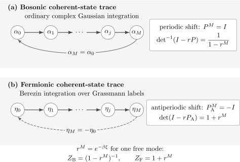
For a free mode, the same one-step factor $r=e^{-\epsilon_\tau\xi/\hbar}$ enters both traces. Ordinary complex integration over a periodic chain gives an inverse determinant and the Bose factor. Berezin integration over an antiperiodic chain gives a determinant and the Fermi factor.

Boundary Conditions and Matsubara Frequencies

Periodic bosonic labels have the Fourier expansion

$$\alpha(\tau) = \sum_{n\in\mathbb Z} \alpha_n e^{-i\nu_n\tau},$$

with

$$\nu_n = \frac{2\pi n}{\beta\hbar}.$$

Antiperiodic fermionic labels have

$$\eta(\tau) = \sum_{n\in\mathbb Z} \eta_n e^{-i\omega_n\tau},$$

where

$$\omega_n = \frac{(2n+1)\pi}{\beta\hbar}.$$

For the free actions, the frequency-space kernels are

$$\begin{aligned} \mathcal D_{\mathrm B}(i\nu_n) &= -i\hbar\nu_n+\xi, \\ \mathcal D_{\mathrm F}(i\omega_n) &= -i\hbar\omega_n+\xi. \end{aligned}$$

Bosons have a zero-frequency mode; fermions do not. The difference is fixed by the thermal trace, not by assigning a different temperature to the two systems.

Bosonic and Fermionic Matsubara Frequencies owns the full frequency grid, finite-cutoff pairing, zero-mode treatment, and convention checks.

From Modes to Nonrelativistic Fields

For finitely many bosonic modes, consider

$$\begin{aligned} \mathcal K &= \sum_{ij} h_{ij}b_i^\dagger b_j \\ &\quad+ \frac{1}{2} \sum_{ijkl} V_{ij;kl} b_i^\dagger b_j^\dagger b_l b_k. \end{aligned}$$

Its normal symbol is

$$\begin{aligned} \mathcal K_{\mathrm N} &= \sum_{ij} h_{ij}\alpha_i^*\alpha_j \\ &\quad+ \frac{1}{2} \sum_{ijkl} V_{ij;kl} \alpha_i^*\alpha_j^* \alpha_l\alpha_k. \end{aligned}$$

The action is

$$S_{\mathrm B} = \int_0^{\beta\hbar} d\tau\, \left[ \hbar \sum_i \alpha_i^*\partial_\tau\alpha_i + \mathcal K_{\mathrm N} \right].$$

Choose spatial basis functions $\varphi_i(\mathbf x)$ and define

$$\psi(\mathbf x,\tau) = \sum_i \varphi_i(\mathbf x)\alpha_i(\tau).$$

The mode sum then becomes a regulated complex field integral. For a common nonrelativistic bosonic model,

$$\begin{aligned} S_{\mathrm B} &= \int_0^{\beta\hbar} d\tau \int d^d x \\ &\quad\times \Bigg[ \hbar\psi^*\partial_\tau\psi + \psi^* \left( -\frac{\hbar^2\nabla^2}{2m} -\mu \right) \psi \\ &\qquad\qquad+ \frac{g}{2} (\psi^*\psi)^2 \Bigg]. \end{aligned}$$

Here $\psi$ is a coherent-state integration variable. It is not generally a normalized one-particle wavefunction, even though a saddle point may obey an equation resembling a nonlinear Schrödinger equation.

Fermionic modes produce the parallel Grassmann field

$$\psi(\mathbf x,\tau) = \sum_i \varphi_i(\mathbf x)\eta_i(\tau),$$

with antiperiodic time boundary conditions. Multi-flavor quartic products need not vanish because they contain distinct Grassmann generators.

Normal Ordering Is Not Optional

The substitution

$$a^\dagger \mapsto \alpha^*, \qquad a \mapsto \alpha$$

is valid for the normal-ordered symbol, not for an arbitrary printed operator string.

Reversing Two Operators

For a boson,

$$aa^\dagger = a^\dagger a+1.$$

Its normal symbol is therefore

$$\alpha^*\alpha+1,$$

not merely $\alpha^*\alpha$. Dropping the constant changes the partition function by an exponential factor.

Squaring the Number Operator

For a bosonic number operator $n=a^\dagger a$,

$$n^2 = (a^\dagger)^2a^2 + a^\dagger a.$$

Thus

$$(n^2)_{\mathrm N} = (\alpha^*\alpha)^2 + \alpha^*\alpha.$$

The naive square of the symbol of $n$ misses the linear term.

For one fermionic mode,

$$n^2 = n.$$

The Grassmann monomial

$$(\bar\eta\eta)^2 = 0$$

does not mean that $n^2$ vanishes. Normal ordering first gives the correct linear symbol $\bar\eta\eta$.

A Naturally Normal-Ordered Interaction

The single-mode bosonic interaction

$$\frac{U}{2}n(n-1) = \frac{U}{2} (a^\dagger)^2a^2$$

has symbol

$$\frac{U}{2} (\alpha^*\alpha)^2.$$

This is why the occupation form $n(n-1)$ is especially convenient in coherent-state treatments.

Several Symbols Exist

For an operator $A$, commonly encountered phase-space symbols include:

• the off-diagonal normal symbol selected by the time-sliced matrix element;
• the diagonal expectation or covariant symbol $\langle\alpha|A|\alpha\rangle$;
• a contravariant symbol in an expansion of $A$ over coherent-state projectors;
• the Weyl symbol associated with symmetric ordering.

They differ by commutator corrections. For example, the normal and Weyl symbols of a quadratic oscillator Hamiltonian differ by a zero-point constant. For nonlinear operators the difference can include lower-degree terms and finite corrections.

Writing

$$S = \int d\tau\, \left( \hbar\alpha^*\dot\alpha + H(\alpha^*,\alpha) \right)$$

without declaring which $H$ appears is incomplete.

Why the Finite-Slice Rule Matters

An expression that is of order $\epsilon_\tau$ on each slice can accumulate over

$$M = \frac{\beta\hbar}{\epsilon_\tau}$$

slices into a finite contribution. This is the core reason a seemingly harmless continuum replacement can fail.

A safe derivation follows this order:

1. choose normalized or unnormalized coherent states;
2. fix the resolution of identity and measure order;
3. write the exact trace formula;
4. preserve adjacent-slice arguments;
5. identify the operator symbol;
6. take the continuum limit only after the finite product is controlled;
7. test the result against a spectral sum or exact determinant.

Continuum coherent-state path integrals have known counterexamples when nonlinear Hamiltonians are assigned an inconsistent symbol or when the time lattice is discarded too early. The existence of a plausible first-order action is not enough to prove equivalence with the operator theory.

Open Kernels and Endpoint Data

For a thermal trace, labels close periodically or antiperiodically. An open coherent-state kernel has different endpoint logic.

The action is first order in time. In a holomorphic convention, one naturally fixes an initial annihilation label and a final creation label, rather than independently fixing both $\alpha$ and $\alpha^*$ at both endpoints. Boundary terms complete the variational problem.

This is unlike a second-order coordinate action, where fixing initial and final positions is natural. Copying coordinate boundary conditions into a coherent-state action can overconstrain the saddle-point equations.

Sources and Correlation Functions

For bosons, add ordinary complex sources. Define

$$\begin{aligned} \mathcal I_{\mathrm B} &= \int d\tau\, (\bar J\alpha+\alpha^*J), \\ S_{{\mathrm B},J} &= S_{\mathrm B}-\mathcal I_{\mathrm B}. \end{aligned}$$

Then

$$\begin{aligned} \mathcal Z_{\mathrm B} [\bar J,J] &= \int \mathcal D\alpha^* \mathcal D\alpha e^{-S_{{\mathrm B},J}/\hbar}. \end{aligned}$$

Functional derivatives generate coherent-state field correlators.

For fermions, the sources must themselves be Grassmann odd. Define

$$\begin{aligned} \mathcal I_{\mathrm F} &= \int d\tau\, (\bar\zeta\eta+\bar\eta\zeta), \\ S_{{\mathrm F},\zeta} &= S_{\mathrm F}-\mathcal I_{\mathrm F}. \end{aligned}$$

Then

$$\begin{aligned} \mathcal Z_{\mathrm F} [\bar\zeta,\zeta] &= \int \mathcal D\bar\eta \mathcal D\eta e^{-S_{{\mathrm F},\zeta}/\hbar}. \end{aligned}$$

Left and right Grassmann derivatives carry ordering signs. A fermionic source is an algebraic generator, not an ordinary laboratory force. Thermal Green Functions supplies the operator ordering and equal-time conventions needed to interpret the resulting two-point functions.

Integrating Out Gaussian Fields

For a positive bosonic quadratic form $A$,

$$\int \mathcal D\alpha^* \mathcal D\alpha\, e^{-\alpha^*A\alpha} \propto \det\nolimits^{-1}A.$$

For a fermionic quadratic form $D$,

$$\int \mathcal D\bar\eta \mathcal D\eta\, e^{-\bar\eta D\eta} \propto \det D.$$

This compact difference drives much of perturbative and numerical field theory. After fermions are integrated out, their determinant depends on any remaining bosonic or auxiliary fields.

The determinant need not be positive. A negative or complex fermion determinant creates a sign or phase problem for stochastic sampling. Grassmann integration itself is exact algebra; the numerical difficulty appears after the result is represented using ordinary numbers.

Physical Interpretation

Coherent-state fields are best understood as integration coordinates on Fock space.

• A bosonic label tracks an annihilation-operator eigenvalue, not a directly measured classical amplitude.
• A fermionic label is nilpotent and has no ordinary numerical value.
• A saddle point can identify a useful mean field without turning the exact path integral into a classical theory.
• Fluctuations around a saddle encode quantum and thermal corrections.
• Symmetry breaking at finite regulator and volume requires the usual source and limiting procedures; a nonzero saddle alone is not an exact finite-system order parameter.

The construction is especially effective because second-quantized Hamiltonians become local polynomials in the coherent-state fields. Its convenience does not erase the Hilbert-space operator origin.

Bridge to Field Theory

A finite-mode coherent-state path integral is an exact reformulation of a regulated many-body trace when its discretization and symbols are correct. Passing to a continuum field theory adds new questions:

• how spatial ultraviolet modes are regulated;
• whether couplings require renormalization;
• how gauge redundancy and constraints are handled;
• which observables survive the continuum limit;
• whether a Euclidean theory reconstructs a unitary Lorentzian theory;
• how anomalies or topological terms modify the measure.

Nonrelativistic many-body fields already use field-theoretic mathematics, but relativistic QFT adds locality, antiparticles, relativistic symmetry, vacuum structure, and renormalization as central principles. Nonrelativistic Field Theory from Many-Body QM develops the Lorentzian action, conserved current, propagator, and contact-EFT matching. Why Many-Body QM Leads to QFT and From Euclidean Time to Euclidean QFT make the wider conceptual boundary explicit.

Common Mistakes

1. Treating coherent states as an orthogonal basis. Their overlap is nonzero, and their identity resolution is overcomplete.
2. Replacing every operator string by commuting numbers. Reorder first and declare the symbol.
3. Discarding adjacent-slice arguments. They encode the normal symbol and the first-order derivative.
4. Guessing fermionic antiperiodicity. Derive it from the graded trace formula.
5. Using ordinary complex variables for fermions. That loses nilpotency, anticommutation, and determinant signs.
6. Calling a Berezin integral a probability average. It is an algebraic coefficient-extraction rule.
7. Forgetting bosonic convergence. A free bosonic grand-canonical mode requires a positive excitation energy.
8. Fixing both complex endpoint variables in an open first-order action. This can overconstrain the boundary-value problem.
9. Equating a saddle field with an exact expectation value. Saddle points are approximations unless a controlled limit makes them exact.
10. Ignoring zero-point and ordering constants. They change absolute partition functions and free energies.
11. Assuming a fermion determinant is positive. It may be signed or complex.
12. Removing the time lattice before checking a nonlinear benchmark. Formal smoothness does not guarantee the correct operator answer.

Working Checklist

Before trusting a coherent-state path integral, record:

• the operator $\mathcal K$ and ensemble;
• bosonic or fermionic statistics for every mode;
• coherent-state normalization;
• overlap and identity resolution;
• Berezin measure order for fermions;
• trace formula and thermal boundary condition;
• finite-slice action with adjacent-slice arguments;
• Hamiltonian symbol and ordering convention;
• spatial and temporal regulators;
• exact free-mode or small-Hilbert-space benchmark;
• convergence, determinant-sign, and continuum-limit diagnostics.

Connections

• Creation and Annihilation Operators supplies the Fock-space algebra.
• Fock Space supplies the variable-particle-number Hilbert space.
• Coherent States develops the one-mode quantum states represented by $\alpha$.
• Coherent States in Phase Space develops the ordinary complex phase-space geometry.
• Path Integrals for Statistical Mechanics provides the coordinate-path comparison and first-quantized exchange sectors.
• Path Integrals for Many-Body Systems places coherent fields beside worldline and local-basis representations and compares their evaluation strategies.
• Coherent-State Path Integrals continues from finite thermal slices to Berry one-forms, mixed endpoints, spin geometry, and field actions.
• Matsubara Formalism Preview develops compact-time Fourier methods.
• Normal Ordering in Many-Body QM develops reference-dependent reorganization beyond the empty vacuum.
• Nonrelativistic Field Theory from Many-Body QM supplies the regulated continuum action and contact-interaction matching.
• Phase-Space QM to QFT compares canonical, coherent-state, and field phase spaces.

References

1. F. A. Berezin, The Method of Second Quantization, Academic Press (1966) – Grassmann algebra, fermionic coherent states, and second-quantized functional methods.
2. J. R. Klauder and B.-S. Skagerstam, Coherent States: Applications in Physics and Mathematical Physics, World Scientific (1985) – coherent-state representations, geometry, and path integrals.
3. I. Daubechies and J. R. Klauder, “Quantum-Mechanical Path Integrals with Wiener Measure for All Polynomial Hamiltonians. II”, Journal of Mathematical Physics 26, 2239–2256 (1985) – regulated coherent-state path integrals and mathematical control.
4. J. W. Negele and H. Orland, Quantum Many-Particle Systems, CRC Press (2018 reissue) – bosonic and fermionic coherent-state functional integrals in many-body theory.
5. A. Altland and B. Simons, Condensed Matter Field Theory, Cambridge University Press (2010) – finite-temperature functional methods, Grassmann fields, and effective actions.
6. P. Coleman, Introduction to Many-Body Physics, Cambridge University Press (2015) – coherent-state fields and modern many-body applications.
7. J. H. Wilson and V. Galitski, “Breakdown of the Coherent State Path Integral: Two Simple Examples”, Physical Review Letters 106, 110401 (2011) – explicit warning that naive continuum coherent-state prescriptions can fail.

Exercises

1. Bosonic Overlap Product

For normalized coherent states, define $\Delta\alpha_j=\alpha_{j+1}-\alpha_j$ and

$$\mathcal O_{\mathrm{cyc}} = \prod_{j=0}^{M-1} \langle\alpha_{j+1}|\alpha_j\rangle.$$

Prove that a periodic chain satisfies

$$\mathcal O_{\mathrm{cyc}} = \exp\left[ -\sum_{j=0}^{M-1} \alpha_{j+1}^* \Delta\alpha_j \right].$$

Solution

The logarithm of the overlap product is

$$\begin{aligned} \Sigma &= \sum_j \left[ -\frac{|\alpha_{j+1}|^2}{2} -\frac{|\alpha_j|^2}{2} + \alpha_{j+1}^*\alpha_j \right]. \end{aligned}$$

Periodicity permits a cyclic relabeling:

$$\sum_j|\alpha_{j+1}|^2 = \sum_j|\alpha_j|^2.$$

Therefore

$$\begin{aligned} \Sigma &= -\sum_j|\alpha_{j+1}|^2 + \sum_j\alpha_{j+1}^*\alpha_j \\ &= -\sum_j \alpha_{j+1}^* (\alpha_{j+1}-\alpha_j). \end{aligned}$$

Exponentiating gives the stated identity. The discrete derivative term comes entirely from nonorthogonal overlaps.

2. Bosonic Free-Mode Determinant

Let $P$ be the $M\times M$ periodic shift matrix and $r=e^{-\beta\xi/M}$. Show that

$$\det(I-rP) = 1-r^M$$

and recover the free bosonic partition function.

Solution

The eigenvalues of $P$ are

$$\lambda_n = e^{2\pi i n/M}, \qquad n=0,\ldots,M-1.$$

Hence

$$\det(I-rP) = \prod_{n=0}^{M-1} (1-r\lambda_n).$$

The roots $\lambda_n$ satisfy

$$x^M-1 = \prod_n(x-\lambda_n).$$

Setting $x=1/r$ and multiplying by $r^M$ gives

$$\prod_n(1-r\lambda_n) = 1-r^M.$$

Ordinary complex Gaussian integration inverts the determinant:

$$\mathcal Z_{\mathrm B} = \frac{1}{1-r^M} = \frac{1}{1-e^{-\beta\xi}}.$$

3. Verify the Graded Trace Sign

Using the fermionic trace formula, explain why the endpoint identification is antiperiodic rather than periodic.

Solution

The trace is

$$\operatorname{Tr}A = \int d\bar\eta\,d\eta\, e^{-\bar\eta\eta} \langle-\bar\eta|A|\eta\rangle.$$

After inserting intermediate coherent-state resolutions, the ket label at the start of the chain is $\eta_0$, while the bra label that closes the chain is its negative. Encoding that closing matrix element using the same nearest-neighbor notation requires

$$\eta_M = -\eta_0.$$

The dual label obeys the same antiperiodic rule. The sign is a consequence of evaluating a Fock-space trace with odd coherent labels; it is not an extra dynamical phase.

4. Fermionic Free-Mode Determinant

Let $P_{\mathrm A}$ be an antiperiodic shift satisfying $P_{\mathrm A}^M=-I$. Show that

$$\det(I-rP_{\mathrm A}) = 1+r^M.$$

Solution

Every eigenvalue obeys

$$\lambda_n^M = -1.$$

They are the roots of

$$x^M+1.$$

Therefore

$$\begin{aligned} \det(I-rP_{\mathrm A}) &= \prod_n(1-r\lambda_n) \\ &= 1+r^M. \end{aligned}$$

Berezin integration produces this determinant directly, so

$$\mathcal Z_{\mathrm F} = 1+e^{-\beta\xi}.$$

The two terms are the empty and occupied states.

5. Ordering Audit

Find the normal symbols of $aa^\dagger$, $n^2$, and $n(n-1)$ for one bosonic mode.

Solution

The commutator gives

$$aa^\dagger = a^\dagger a+1,$$

so

$$(aa^\dagger)_{\mathrm N} = \alpha^*\alpha+1.$$

Next,

$$n^2 = (a^\dagger)^2a^2 + a^\dagger a,$$

hence

$$(n^2)_{\mathrm N} = (\alpha^*\alpha)^2 + \alpha^*\alpha.$$

Finally,

$$n(n-1) = (a^\dagger)^2a^2,$$

so

$$\big(n(n-1)\big)_{\mathrm N} = (\alpha^*\alpha)^2.$$

The three examples show why operator reordering must precede substitution.

6. Thermal Frequency Grids

Derive the bosonic and fermionic Matsubara frequencies directly from their coherent-state boundary conditions.

Solution

For a mode $e^{-i\omega\tau}$, periodicity requires

$$e^{-i\omega\beta\hbar} = 1.$$

Thus

$$\omega = \frac{2\pi n}{\beta\hbar}.$$

Antiperiodicity requires

$$e^{-i\omega\beta\hbar} = -1,$$

so

$$\omega = \frac{(2n+1)\pi}{\beta\hbar}.$$

The bosonic grid includes $n=0$ as a zero mode. The fermionic grid is shifted by half a spacing and has no zero mode.

7. One Fermion and Nilpotency

Show that $n^2=n$ for one fermionic mode. Why does the vanishing of $(\bar\eta\eta)^2$ not contradict this result?

Solution

Using

$$aa^\dagger = 1-a^\dagger a,$$

one finds

$$\begin{aligned} n^2 &= a^\dagger a a^\dagger a \\ &= a^\dagger (1-a^\dagger a) a \\ &= a^\dagger a, \end{aligned}$$

because $(a^\dagger)^2=a^2=0$. Therefore $n^2=n$.

The Grassmann square

$$(\bar\eta\eta)^2 = 0$$

would be the result of naively squaring the symbol before normal ordering. The operator identity must be simplified first. Its correct normal symbol is the linear monomial $\bar\eta\eta$.

8. Spatial Field Dimensions

Suppose orthonormal basis functions satisfy

$$\int d^d x\, \varphi_i^*(\mathbf x) \varphi_j(\mathbf x) = \delta_{ij},$$

and

$$\psi(\mathbf x,\tau) = \sum_i \varphi_i(\mathbf x)\alpha_i(\tau).$$

If $\alpha_i$ is dimensionless, determine the spatial dimension of $\psi$ and verify that

$$\int d^d x\, \psi^*\psi$$

is dimensionless.

Solution

Orthonormality requires

$$[\varphi_i] = L^{-d/2}.$$

Since $\alpha_i$ is dimensionless,

$$[\psi] = L^{-d/2}.$$

Therefore

$$[\psi^*\psi] = L^{-d},$$

and multiplication by $d^d x$ gives a dimensionless mode-counting quantity. In second-quantized language, the same dimensional assignment makes

$$\int d^d x\,\psi^*\psi$$

the coherent-state symbol of particle number.