Bosonic and Fermionic Matsubara Frequencies

Matsubara frequencies are the Fourier modes allowed by thermal boundary conditions on compact imaginary time.

For inverse temperature

$$\beta = \frac1{k_{\mathrm B}T},$$

the Matsubara energies are

$$\begin{aligned} \Omega_m &= \frac{2\pi m}{\beta} && \text{bosonic}, \\ \nu_n &= \frac{(2n+1)\pi}{\beta} && \text{fermionic}, \end{aligned}$$

with $m,n\in\mathbb Z$. The corresponding angular frequencies are

$$\begin{aligned} \omega_m^{\mathrm B} &= \frac{2\pi m}{\beta\hbar}, \\ \omega_n^{\mathrm F} &= \frac{(2n+1)\pi}{\beta\hbar}. \end{aligned}$$

Bosons include a zero mode. Fermions are shifted by half a grid spacing and do not.

Canonical Scope

This page is the canonical reference for:

• bosonic and fermionic Matsubara energy grids;
• explicit-$\hbar$ angular-frequency conventions;
• the natural-unit variants;
• the boundary-condition derivation;
• negative-index identities and symmetric summation;
• assignment by total fermion parity;
• zero modes, minimum frequencies, and temperature spacing;
• frequency arithmetic at vertices;
• finite-grid and discrete-Fourier-transform conventions;
• simple twisted thermal boundary conditions.

Matsubara Formalism Preview owns the complete equilibrium calculation workflow, transform derivation, loop sums, convergence prescriptions, and QFT handoff. Green Functions in Many-Body QM owns single-particle propagator and spectral conventions. Diagrammatic Methods Preview owns line, vertex, self-energy, and diagrammatic rules.

Quick Lookup

Quantity	Bosonic channel	Fermionic channel
boundary condition	$F(\tau+\beta\hbar)=F(\tau)$	$F(\tau+\beta\hbar)=-F(\tau)$
Matsubara energy	$\Omega_m=2\pi m/\beta$	$\nu_n=(2n+1)\pi/\beta$
angular frequency	$\omega_m^{\mathrm B}=2\pi m/(\beta\hbar)$	$\omega_n^{\mathrm F}=(2n+1)\pi/(\beta\hbar)$
grid spacing	$2\pi/\beta$	$2\pi/\beta$
nearest point to zero	$\Omega_0=0$	$\nu_{-1}=-\pi/\beta$, $\nu_0=\pi/\beta$
negative-index identity	$\Omega_{-m}=-\Omega_m$	$\nu_{-n-1}=-\nu_n$
zero mode	present	absent
typical channel	density, spin, current, pair field	single creation or annihilation field

The argument of a Matsubara Green function is normally written $i\Omega_m$ or $i\nu_n$. The factor $i$ identifies a point on the imaginary axis of a complex-energy plane; it is not part of the real number $\Omega_m$ or $\nu_n$ itself.

Notation Ledger

This page keeps four distinct objects:

Symbol	Meaning	Units
$\beta$	inverse temperature	inverse energy
$L_\tau=\beta\hbar$	thermal circumference	time
$\Omega_m$, $\nu_n$	Matsubara energies	energy
$\omega_m^{\mathrm B}$, $\omega_n^{\mathrm F}$	angular Matsubara frequencies	inverse time

The conversions are

$$\begin{aligned} \Omega_m &= \hbar\omega_m^{\mathrm B}, \\ \nu_n &= \hbar\omega_n^{\mathrm F}. \end{aligned}$$

In terms of temperature,

$$\begin{aligned} \Omega_m &= 2\pi m\,k_{\mathrm B}T, \\ \nu_n &= (2n+1)\pi k_{\mathrm B}T. \end{aligned}$$

Why use separate letters?

Many texts use $\omega_n$ for both grids and rely on context. This page uses:

• $\Omega_m$ for a bosonic Matsubara energy;
• $\nu_n$ for a fermionic Matsubara energy.

The distinction makes expressions such as

$$\nu_n+\Omega_m$$

visibly fermionic and reduces index-routing errors.

Boundary-Condition Origin

Let the thermal circumference be

$$L_\tau = \beta\hbar.$$

A Fourier mode is

$$f_\zeta(\tau) = e^{-i\zeta\tau/\hbar},$$

where $\zeta$ has energy units.

Periodic channel

For

$$f_\zeta(\tau+L_\tau) = f_\zeta(\tau),$$

one requires

$$e^{-i\beta\zeta} = 1.$$

Thus

$$\beta\zeta = 2\pi m,$$

which gives

$$\Omega_m = \frac{2\pi m}{\beta}.$$

Antiperiodic channel

For

$$f_\zeta(\tau+L_\tau) = -f_\zeta(\tau),$$

one requires

$$e^{-i\beta\zeta} = -1.$$

Therefore

$$\beta\zeta = (2n+1)\pi,$$

which gives

$$\nu_n = \frac{(2n+1)\pi}{\beta}.$$

The sign ultimately comes from trace cyclicity combined with graded imaginary-time ordering. It does not mean that a physical fermion state evolves for a time $\beta\hbar$ and literally returns with a minus sign.

The Two Grids

Define the common spacing

$$\Delta\nu := \frac{2\pi}{\beta}.$$

Then

$$\begin{aligned} \Omega_m &= m\Delta\nu, \\ \nu_n &= \left( n+\frac12 \right) \Delta\nu. \end{aligned}$$

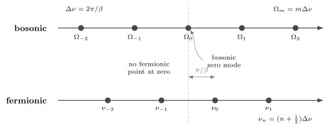
Bosonic and fermionic Matsubara energy grids. Both have spacing $\Delta\nu=2\pi/\beta$, but the fermionic grid is displaced by $\Delta\nu/2=\pi/\beta$. Divide by $\hbar$ to obtain angular frequencies.

Bosonic sequence

Around the origin,

$$\ldots, -\frac{4\pi}{\beta}, -\frac{2\pi}{\beta}, 0, \frac{2\pi}{\beta}, \frac{4\pi}{\beta}, \ldots$$

corresponds to

$$\ldots, \Omega_{-2}, \Omega_{-1}, \Omega_0, \Omega_1, \Omega_2, \ldots$$

Fermionic sequence

Around the origin,

$$\ldots, -\frac{3\pi}{\beta}, -\frac{\pi}{\beta}, \frac{\pi}{\beta}, \frac{3\pi}{\beta}, \ldots$$

corresponds to

$$\ldots, \nu_{-2}, \nu_{-1}, \nu_0, \nu_1, \ldots$$

The labels nearest zero are $n=-1$ and $n=0$, not $n=0$ and $n=1$.

Index Symmetries

For bosons,

$$\Omega_{-m} = -\Omega_m.$$

For fermions,

$$\nu_{-n-1} = -\nu_n.$$

In particular,

$$\nu_{-1} = -\nu_0 = -\frac{\pi}{\beta}.$$

The tempting identity $\nu_{-n}=-\nu_n$ is false:

$$\nu_{-n} = \frac{(1-2n)\pi}{\beta}.$$

Symmetric sums

If $F$ is even and the sums converge,

$$\sum_{m=-\infty}^{\infty} F(\Omega_m) = F(0) + 2\sum_{m=1}^{\infty} F(\Omega_m),$$

whereas

$$\sum_{n=-\infty}^{\infty} F(\nu_n) = 2\sum_{n=0}^{\infty} F(\nu_n).$$

The fermionic pairing is between indices $n$ and $-n-1$.

For an odd integrand, a symmetric sum may vanish, but only if the summation prescription respects the pairing and the expression is sufficiently convergent or regulated. A shift of a conditionally convergent series can change an intermediate result.

Which Grid Does an Operator Use?

The grid is determined by the total fermion parity of the operator channel.

Let

$$\begin{aligned} (-1)^N O(-1)^N &= (-1)^{p_O}O, \\ p_O &\in \{0,1\}. \end{aligned}$$

Then:

$$\begin{aligned} p_O=0 &\Longrightarrow \text{bosonic grid}, \\ p_O=1 &\Longrightarrow \text{fermionic grid}. \end{aligned}$$

Common assignments

Operator	Number of odd fermionic factors modulo two	Grid
$c_i$ or $c_i^\dagger$	1	fermionic
$c_i^\dagger c_j$	0	bosonic
density $n_i$	0	bosonic
spin density	0	bosonic
current	0	bosonic
pair field $c_{i\downarrow}c_{i\uparrow}$	0	bosonic
three-fermion composite	1	fermionic
elementary boson field $b_i$	0	bosonic

A pair field is built from fermions but is even. Its pair susceptibility therefore carries a bosonic external Matsubara energy and may have an $\Omega_0$ component.

Green functions versus observables

A normal single-particle fermion Green function is antiperiodic in the difference of its time arguments. A density-density, spin-spin, or current-current correlator is periodic. The statistics of an internal line and the statistics of the external response channel need not match.

Frequency Arithmetic

The grids obey:

$$\begin{aligned} \Omega_m+\Omega_\ell &= \Omega_{m+\ell}, \\ \nu_n+\Omega_m &= \nu_{n+m}, \\ \nu_n-\nu_r &= \Omega_{n-r}. \end{aligned}$$

These identities encode parity conservation:

• boson plus boson gives boson;
• fermion plus boson gives fermion;
• fermion minus fermion gives boson.

For a density bubble with external $\Omega_\ell$, the two internal fermionic arguments may be

$$i\nu_n \qquad \text{and} \qquad i\nu_n+i\Omega_\ell.$$

The second lies on the fermionic grid because

$$\nu_n+\Omega_\ell = \nu_{n+\ell}.$$

Zero Modes

The bosonic grid contains

$$\Omega_0 = 0.$$

This mode represents a configuration constant around the thermal circle. It is often important for:

• static susceptibilities;
• order-parameter fluctuations;
• long-distance thermal behavior;
• dimensional-reduction arguments;
• infrared divergences near criticality.

The existence of a zero frequency does not imply a divergent propagator. A denominator such as

$$\Omega_m^2+E^2$$

remains finite at $m=0$ when $E>0$. Divergence requires additional infrared structure, such as a vanishing mass or gap.

No fermionic zero mode

The nearest fermionic energies are

$$\nu_{-1} = -\frac{\pi}{\beta}, \qquad \nu_0 = \frac{\pi}{\beta}.$$

At nonzero temperature, an odd thermal field therefore has a smallest Matsubara-energy magnitude $\pi/\beta$.

This does not mean that a fermionic system cannot have a zero-energy excitation after analytic continuation. It means only that the discrete imaginary-energy sampling grid has no point at zero for an antiperiodic channel.

Temperature and Grid Spacing

The common spacing is

$$\Delta\nu = \frac{2\pi}{\beta} = 2\pi k_{\mathrm B}T.$$

The smallest nonzero magnitudes are

$$\begin{aligned} \lvert\Omega_{\pm1}\rvert &= 2\pi k_{\mathrm B}T, \\ \lvert\nu_{-1}\rvert = \lvert\nu_0\rvert &= \pi k_{\mathrm B}T. \end{aligned}$$

As $T\to0$,

$$\Delta\nu \longrightarrow 0,$$

and both grids become dense on the imaginary-energy axis.

As temperature increases, the points spread farther apart. Fewer low-energy samples then lie within a fixed physical bandwidth, while the bosonic zero mode remains at the origin.

Energy and Angular-Frequency Conventions

Two internally consistent transform conventions are common.

Energy convention

Use $\zeta_n=\hbar\omega_n$ and

$$F_E(i\zeta_n) = \frac1\hbar \int_0^{\beta\hbar} d\tau\, e^{i\zeta_n\tau/\hbar} F(\tau).$$

The inverse is

$$F(\tau) = \frac1\beta \sum_n e^{-i\zeta_n\tau/\hbar} F_E(i\zeta_n).$$

The sum measure is $1/\beta$ times a discrete sum.

Angular-frequency convention

Use $\omega_n=\zeta_n/\hbar$ and

$$F_\omega(i\omega_n) = \int_0^{\beta\hbar} d\tau\, e^{i\omega_n\tau} F(\tau).$$

The inverse is

$$F(\tau) = \frac1{\beta\hbar} \sum_n e^{-i\omega_n\tau} F_\omega(i\omega_n).$$

For the same time-domain function,

$$F_\omega(i\omega_n) = \hbar F_E(i\zeta_n).$$

Mixing the forward transform from one convention with the inverse normalization from the other produces a missing or extra factor of $\hbar$.

Natural Units

If

$$\hbar = k_{\mathrm B} = 1,$$

then

$$\beta = \frac1T, \qquad 0\leq\tau<\beta,$$

and

$$\begin{aligned} \Omega_m &= 2\pi mT, \\ \nu_n &= (2n+1)\pi T. \end{aligned}$$

Energy, inverse time, and temperature share the same units. This convenience hides which factors must be restored.

If only $k_{\mathrm B}=1$ but $\hbar$ remains explicit, then $\beta=1/T$ while the thermal circumference is still $\beta\hbar$ and angular frequencies still carry $1/\hbar$.

Sum Measures

In energy notation, a thermal loop sum is written

$$\frac1\beta \sum_n F(i\zeta_n).$$

In angular-frequency notation, the corresponding measure is

$$\frac1{\beta\hbar} \sum_n F(i\omega_n).$$

At zero temperature, under suitable convergence assumptions,

$$\frac1\beta \sum_n F(i\zeta_n) \longrightarrow \int_{-\infty}^{\infty} \frac{d\zeta}{2\pi} F(i\zeta).$$

The detailed use of these sums, including convergence factors and contour methods, belongs to Matsubara Formalism Preview.

Imaginary-Axis Labels and Analytic Continuation

The label $G(i\zeta_n)$ means that a function is sampled at discrete points on the imaginary-energy axis. It does not make $i\zeta_n$ a physical real frequency. A retarded function is obtained only after identifying an analytic function with the correct spectral and growth properties and taking the boundary value

$$i\zeta_n \longrightarrow \omega+i0^+,$$

with units adjusted to the chosen energy or angular-frequency convention. The advanced boundary value uses $\omega-i0^+$. Finite noisy Matsubara data generally do not determine this continuation stably without additional information or regularization.

Chemical Potential

For a grand-canonical ensemble,

$$\mathcal K = H-\mu N.$$

In the standard convention, the bosonic or fermionic grid remains fixed by thermal boundary conditions. The chemical potential enters the operator evolution and propagator denominator through energies measured relative to $\mu$.

For a free fermionic mode,

$$\xi = \epsilon-\mu,$$

and the normal propagator has the form

$$\mathcal G_0(i\nu_n) = \frac1{i\nu_n-\xi}.$$

One should not replace the standard grid by $\nu_n-\mu$ without also changing the convention for the thermal boundary condition and time evolution.

Twisted Thermal Boundary Conditions

A useful generalization is

$$F(\tau+\beta\hbar) = e^{-i\theta} F(\tau),$$

where $\theta$ is defined modulo $2\pi$. The mode condition becomes

$$e^{-i\beta\zeta} = e^{-i\theta},$$

so

$$\zeta_n(\theta) = \frac{2\pi n+\theta}{\beta}.$$

The standard cases are:

$$\begin{aligned} \theta=0 &\Longrightarrow \text{periodic bosonic grid}, \\ \theta=\pi &\Longrightarrow \text{antiperiodic fermionic grid}. \end{aligned}$$

Twists arise in boundary-condition probes, imaginary chemical potentials, and thermal holonomies. Gauge equivalence, charge assignments, and analytic continuation in chemical potential require additional care; the standard formulas on this page assume $\theta=0$ or $\pi$.

Numerical Frequency Grids

A computation truncates the infinite grid. The truncation must preserve the symmetry appropriate to the channel.

Bosonic finite grid

For a symmetric cutoff $M$,

$$m = -M,\ldots,M$$

contains $2M+1$ points and includes $m=0$.

Fermionic finite grid

A symmetric frequency set may use

$$n = -M,\ldots,M-1.$$

It contains $2M$ points paired by

$$n \longleftrightarrow -n-1.$$

The set includes both $\nu_{-1}=-\pi/\beta$ and $\nu_0=\pi/\beta$.

Discrete imaginary time

If imaginary time is sampled at $N_\tau$ points, the representable frequency range is finite. The exact ordering of positive and negative indices depends on the discrete-Fourier-transform library. A reliable implementation records:

• whether the time grid includes an endpoint;
• where zero frequency is stored;
• how negative frequencies wrap in array order;
• whether a half-step phase was used for antiperiodic fields;
• the ultraviolet cutoff implied by the time spacing;
• the normalization of both transforms.

Do not infer physical asymmetry from an array whose negative-frequency half has merely been stored after the positive-frequency half.

Worked Scale Example

Let $E_0$ be a reference energy and choose

$$\beta E_0 = 8.$$

Then the spacing in units of $E_0$ is

$$\frac{\Delta\nu}{E_0} = \frac{2\pi}{8} = \frac{\pi}{4}.$$

The nearest fermionic points have magnitude

$$\frac{\lvert\nu_0\rvert}{E_0} = \frac{\pi}{8}.$$

Thus the first points are:

Channel	Negative point	Zero	Positive point
bosonic	$\Omega_{-1}/E_0=-\pi/4$	$\Omega_0=0$	$\Omega_1/E_0=\pi/4$
fermionic	$\nu_{-1}/E_0=-\pi/8$	none	$\nu_0/E_0=\pi/8$

This example is dimensionless and remains valid for any system once $\beta E_0$ is fixed.

Diagnostic Checklist

When reading or writing a finite-temperature formula, identify:

1. Is the symbol an energy or an angular frequency?
2. Is $\tau$ measured in time or inverse-energy units?
3. Is the channel even or odd under fermion parity?
4. Does the stated grid include a zero mode?
5. Are negative fermionic indices paired as $n$ and $-n-1$?
6. Is the sum measure $1/\beta$ or $1/(\beta\hbar)$?
7. Does a chemical potential enter the generator or an explicitly twisted boundary condition?
8. Are external and internal frequencies on compatible grids?
9. Does a finite cutoff preserve positive-negative pairing?
10. Is a real-frequency statement being inferred only after a valid analytic continuation?

Common Mistakes

• Calling $\nu_n$ an angular frequency while assigning it energy units.
• Forgetting $\hbar$ in $\omega_n=\nu_n/\hbar$.
• Using the fermionic formula for a density, current, spin, or pair channel.
• Assuming every object built from fermion operators is fermionic.
• Writing $\nu_{-n}=-\nu_n$ instead of $\nu_{-n-1}=-\nu_n$.
• Omitting the bosonic $m=0$ term in a symmetric sum.
• Inserting a fictitious fermionic zero mode.
• Interpreting the absence of a fermionic zero Matsubara point as a physical spectral gap.
• Using $1/\beta$ with an angular-frequency transform that requires $1/(\beta\hbar)$.
• Shifting a conditionally convergent sum without preserving its regulator.
• Treating $\mu$ as an automatic real shift of the standard Matsubara grid.
• Confusing a finite FFT array order with increasing signed frequency.
• Setting $\hbar=1$ in one line and restoring it by dimensional guesswork later.

Cross-Links

• Matsubara Frequency Table provides the compact grid, units, parity, routing, and sum-measure lookup.
• Matsubara Formalism Preview develops the full compact-time and frequency-sum workflow.
• Thermal Green Functions applies the grids to graded propagators, equal-time contact terms, and free-mode benchmarks.
• Spectral Representation shows how those grids sample spectral Cauchy transforms and why an exact bosonic static term requires separate zero-mode bookkeeping.
• Imaginary Time explains the thermal circumference and trace construction.
• Finite-Temperature QM Overview maps the chapter’s operator, spectral, and path-integral representations.
• Core Objects and Notation gives the wider many-body symbol ledger.
• Fourier-Transform Conventions owns the site’s general transform conventions.
• Green Functions in Many-Body QM fixes single-particle Matsubara and spectral normalizations.
• Diagrammatic Methods Preview applies the grids to internal lines and vertices.
• From Euclidean Time to Euclidean QFT gives the field-theory realization.

References

1. T. Matsubara, “A New Approach to Quantum-Statistical Mechanics”, Progress of Theoretical Physics 14, 351–378 (1955) – original imaginary-time many-body formalism.
2. P. C. Martin and J. Schwinger, “Theory of Many-Particle Systems. I”, Physical Review 115, 1342–1373 (1959) – equilibrium Green functions and thermal boundary structure.
3. G. Baym and N. D. Mermin, “Determination of Thermodynamic Green’s Functions”, Journal of Mathematical Physics 2, 232–234 (1961) – analytic conditions associated with thermal Green functions.
4. A. L. Fetter and J. D. Walecka, Quantum Theory of Many-Particle Systems, Dover (2003 reprint of the 1971 edition) – many-body finite-temperature conventions.
5. G. D. Mahan, Many-Particle Physics, 3rd ed., Springer (2000) – Matsubara sums and condensed-matter applications.
6. J. W. Negele and H. Orland, Quantum Many-Particle Systems, CRC Press (2018 reissue) – operator and functional finite-temperature methods.
7. M. Le Bellac, Thermal Field Theory, Cambridge University Press (1996) – thermal frequency conventions in relativistic field theory.
8. J. I. Kapusta and C. Gale, Finite-Temperature Field Theory, 2nd ed., Cambridge University Press (2006) – thermal sums, zero modes, and field-theory applications.

Exercises

1. Reconstruct the grids from parity

Suppose a channel obeys

$$\begin{aligned} F_p(\tau+\beta\hbar) &= (-1)^p F_p(\tau), \\ p &\in \{0,1\}. \end{aligned}$$

Derive one formula for its allowed Matsubara energies.

Solution

For a mode $e^{-i\zeta\tau/\hbar}$, the boundary condition requires

$$e^{-i\beta\zeta} = (-1)^p = e^{-i\pi p}.$$

Therefore

$$\beta\zeta = 2\pi n+\pi p,$$

up to an integer relabeling. Hence

$$\zeta_n^{(p)} = \frac{(2n+p)\pi}{\beta}.$$

Setting $p=0$ gives the bosonic grid, while $p=1$ gives the fermionic grid.

2. Match transform normalizations

Starting from the energy convention

$$F(\tau) = \frac1\beta\sum_n e^{-i\zeta_n\tau/\hbar}F(i\zeta_n),$$

set $\zeta_n=\hbar\omega_n$ and define $\widetilde F(i\omega_n)=\hbar F(i\zeta_n)$. Show that the same function can be written with the angular-frequency sum measure $1/(\beta\hbar)$.

Solution

Substitution gives

$$F(\tau) = \frac1\beta\sum_n e^{-i\omega_n\tau} \frac{\widetilde F(i\omega_n)}{\hbar} = \frac1{\beta\hbar}\sum_n e^{-i\omega_n\tau} \widetilde F(i\omega_n).$$

The factor of $\hbar$ therefore moves between the transform coefficient and the frequency-space function. Mixing the exponent from one convention with the normalization of the other changes dimensions.

3. Pair negative fermionic frequencies

Show that the negative of $\nu_n$ is $\nu_{-n-1}$. Use the result to rewrite an even fermionic sum over all integers as a sum over nonnegative $n$.

Solution

By definition,

$$\begin{aligned} \nu_{-n-1} &= \frac{ \left[ 2(-n-1)+1 \right]\pi }{ \beta } \\ &= -\frac{(2n+1)\pi}{\beta} \\ &= -\nu_n. \end{aligned}$$

If $F(-\nu)=F(\nu)$ and the sum converges,

$$\sum_{n=-\infty}^{\infty} F(\nu_n) = 2 \sum_{n=0}^{\infty} F(\nu_n).$$

The nonnegative labels $n\geq0$ represent the positive-frequency half; the matching negative label is $-n-1$.

4. Restore explicit constants

A natural-unit calculation writes

$$\nu_n = (2n+1)\pi T.$$

Restore $k_{\mathrm B}$ and $\hbar$ for both the Matsubara energy and angular frequency.

Solution

Temperature becomes an energy through $k_{\mathrm B}T$. Therefore

$$\nu_n = (2n+1)\pi k_{\mathrm B}T.$$

Dividing by $\hbar$ gives the angular frequency:

$$\omega_n^{\mathrm F} = \frac{ (2n+1)\pi k_{\mathrm B}T }{ \hbar }.$$

The first has energy units; the second has inverse-time units.

5. Classify composite channels

Classify the Matsubara grid for each operator:

$$\begin{aligned} O_1 &= c_i^\dagger c_j, \\ O_2 &= c_i c_j c_k, \\ O_3 &= c_{i\downarrow}c_{i\uparrow}, \\ O_4 &= b_i^\dagger c_j. \end{aligned}$$

Here $b_i$ is bosonic.

Solution

$O_1$ contains two odd factors and is even, so it uses the bosonic grid.

$O_2$ contains three odd factors and is odd, so it uses the fermionic grid.

$O_3$ is a pair field with two odd factors. It is even and uses the bosonic grid.

$O_4$ contains one odd fermionic factor; the bosonic factor does not change fermion parity. It is odd and uses the fermionic grid.

6. Check vertex routing

Let an incoming fermion carry $\nu_n$ and an emitted boson carry $\Omega_m$. Show that the outgoing fermion energy $\nu_n-\Omega_m$ remains on the fermionic grid.

Solution

Directly,

$$\begin{aligned} \nu_n-\Omega_m &= \frac{(2n+1)\pi}{\beta} - \frac{2m\pi}{\beta} \\ &= \frac{ \left[ 2(n-m)+1 \right]\pi }{ \beta } \\ &= \nu_{n-m}. \end{aligned}$$

Subtracting a bosonic frequency shifts the integer label but preserves the half-step offset.

7. Derive a twisted grid

For

$$F(\tau+\beta\hbar) = e^{-i\theta}F(\tau),$$

derive the allowed energies and recover the standard grids at $\theta=0$ and $\theta=\pi$.

Solution

A mode $e^{-i\zeta\tau/\hbar}$ must satisfy

$$e^{-i\beta\zeta} = e^{-i\theta}.$$

Thus

$$\beta\zeta = 2\pi n+\theta,$$

and

$$\zeta_n(\theta) = \frac{2\pi n+\theta}{\beta}.$$

For $\theta=0$, this is $2\pi n/\beta$, the periodic bosonic grid. For $\theta=\pi$, it is $(2n+1)\pi/\beta$, the antiperiodic fermionic grid.

8. Design a symmetric finite cutoff

Construct finite bosonic and fermionic index sets that preserve frequency reflection. State the number of points and whether zero is included.

Solution

For bosons, choose

$$m = -M,\ldots,M.$$

This set has $2M+1$ points, is invariant under $m\mapsto-m$, and includes $m=0$.

For fermions, choose

$$n = -M,\ldots,M-1.$$

This set has $2M$ points and is invariant under

$$n \mapsto -n-1.$$

It contains the pair $n=-1,0$ nearest the origin and has no zero-frequency point.