KMS Condition Preview

The Kubo–Martin–Schwinger condition characterizes thermal equilibrium by relating two operator orderings across an imaginary-time displacement of $\beta\hbar$.

For a finite system, it is the precise correlation identity hidden inside cyclicity of the Gibbs trace. For an infinite system, where a global density operator and partition function may not exist, the same identity becomes a definition of equilibrium in terms of observables, dynamics, and complex-time analyticity.

With

$$\beta = \frac{1}{k_{\mathrm B}T},$$

the KMS condition ties together four statements:

1. correlation functions admit analytic continuation through a thermal strip;
2. the two strip boundaries carry opposite operator orderings;
3. imaginary-time-ordered correlators are periodic or antiperiodic;
4. positive- and negative-frequency processes obey thermal detailed balance.

These are not separate thermal rules. They are different consequences of one equilibrium condition.

Scope and Canonical Ownership

This page owns the KMS condition itself: its finite-system derivation, analytic-strip formulation, physical interpretation, elementary diagnostics, and bridge to algebraic statistical mechanics.

Neighboring pages retain more specialized material:

• Thermal Green Functions owns graded imaginary-time ordering, equal-time jumps, contact terms, and free propagator benchmarks.
• Spectral Representation owns thermal Lehmann kernels and spectral densities.
• Fluctuation–Dissipation Theorem owns the conversion between equilibrium fluctuations and absorptive response.
• Analytic Continuation owns the inverse problem of recovering real-frequency information from imaginary-time data.
• Real-Time Thermal Dynamics Preview owns the loss of KMS closure under general preparations and drives, together with the forward–backward contour response.
• Dynamics as Automorphisms owns the broader C*-dynamical and GNS framework.

The purpose here is to make the shared equilibrium structure explicit without duplicating those derivations.

Conventions

Let $\mathcal K$ be the generator used in the equilibrium ensemble. In a canonical ensemble,

$$\mathcal K=H.$$

In a grand-canonical ensemble with conserved particle number,

$$\mathcal K = H-\mu N, \qquad [H,N]=0.$$

The partition function and Gibbs state are

$$\begin{aligned} \mathcal Z &= \operatorname{Tr} \left(e^{-\beta\mathcal K}\right), \\ \omega_\beta(A) &= \langle A\rangle_\beta = \frac{ \operatorname{Tr} \left(e^{-\beta\mathcal K}A\right) }{\mathcal Z}. \end{aligned}$$

Real-time Heisenberg evolution generated by $\mathcal K$ is

$$\alpha_t(A) = e^{i\mathcal Kt/\hbar} A e^{-i\mathcal Kt/\hbar}.$$

When the continuation exists, replace $t$ by a complex variable $z$:

$$\alpha_z(A) = e^{i\mathcal Kz/\hbar} A e^{-i\mathcal Kz/\hbar}.$$

In particular,

$$\alpha_{t+i\beta\hbar}(A) = e^{-\beta\mathcal K} \alpha_t(A) e^{\beta\mathcal K}.$$

The sign of the imaginary displacement follows from the convention

$$\alpha_t(A) = e^{+i\mathcal Kt/\hbar} A e^{-i\mathcal Kt/\hbar}.$$

Changing the sign in the real-time evolution reflects the analytic strip and changes which boundary is written first. It does not change the physical content.

The KMS Condition at a Glance

For two suitable observables $A$ and $B$, define

$$F_{A,B}(z) = \omega_\beta \left( B\alpha_z(A) \right).$$

The equilibrium correlation function is analytic in the open strip

$$0 \lt \operatorname{Im}z \lt \beta\hbar,$$

continuous on its closure, and has boundary values

$$\begin{aligned} F_{A,B}(t) &= \omega_\beta \left( B\alpha_t(A) \right), \\ F_{A,B}(t+i\beta\hbar) &= \omega_\beta \left( \alpha_t(A)B \right). \end{aligned}$$

Equivalently,

$$\omega_\beta \left( \alpha_t(A)B \right) = \omega_\beta \left( B\alpha_{t+i\beta\hbar}(A) \right).$$

At $t=0$ this becomes the twisted trace identity

$$\omega_\beta(AB) = \omega_\beta \left( B\alpha_{i\beta\hbar}(A) \right).$$

The twist is imaginary-time evolution. An ordinary tracial state would satisfy $\omega(AB)=\omega(BA)$; a finite-temperature state instead moves $A$ around the thermal interval before reversing the order.

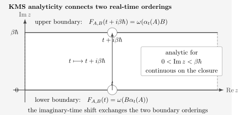
The KMS function is analytic inside the thermal strip. Its lower boundary is $\omega(B\alpha_t(A))$, while its upper boundary is $\omega(\alpha_t(A)B)$. The imaginary displacement $i\beta\hbar$ therefore exchanges the order of $A$ and $B$.

The picture is more informative than a slogan such as “thermal correlators are periodic.” The fundamental statement concerns analytic continuation plus a boundary-order exchange. Periodicity appears only after an ordered correlator is assembled from the two boundaries.

Finite Gibbs Derivation

Assume first that $e^{-\beta\mathcal K}$ is trace class and that the operator products below are well defined. Because $\mathcal K$ commutes with its own evolution,

$$\alpha_{t+i\beta\hbar}(A) = e^{-\beta\mathcal K} \alpha_t(A) e^{\beta\mathcal K}.$$

Equivalently,

$$e^{-\beta\mathcal K}\alpha_t(A) = \alpha_{t+i\beta\hbar}(A) e^{-\beta\mathcal K}.$$

Now cycle the trace and use this operator identity:

$$\begin{aligned} \left\langle \alpha_t(A)B \right\rangle_\beta &= \frac1{\mathcal Z} \operatorname{Tr} \left[ e^{-\beta\mathcal K} \alpha_t(A)B \right] \\ &= \frac1{\mathcal Z} \operatorname{Tr} \left[ B e^{-\beta\mathcal K} \alpha_t(A) \right] \\ &= \frac1{\mathcal Z} \operatorname{Tr} \left[ B\alpha_{t+i\beta\hbar}(A) e^{-\beta\mathcal K} \right] \\ &= \left\langle B\alpha_{t+i\beta\hbar}(A) \right\rangle_\beta. \end{aligned}$$

Nothing in this derivation assumes that $A$ and $B$ commute. Nothing inserts a fermionic minus sign. The only algebraic input is trace cyclicity.

For a finite-dimensional Hilbert space, $F_{A,B}(z)$ is a finite sum of exponentials and is entire in $z$. The KMS strip is then not the maximal analytic domain; it is the domain whose two boundaries encode the equilibrium exchange relation.

For an infinite-dimensional system, analyticity is more delicate. A Gibbs operator may be trace class while unbounded observables require domain control. In algebraic statistical mechanics one works first with bounded observables and states as positive linear functionals, making the strip condition part of the definition rather than an informal continuation of unbounded products.

What the Thermal Shift Means

The transformation

$$A \longmapsto \alpha_{i\beta\hbar}(A) = e^{-\beta\mathcal K} A e^{\beta\mathcal K}$$

is not unitary evolution. It is similarity transformation through an imaginary-time interval. In the Gibbs trace, that transformation supplies exactly the factors needed to move $A$ past the thermal weight.

There are three complementary interpretations.

Operator interpretation

The insertion $A$ is transported once through the Gibbs factor:

$$e^{-\beta\mathcal K}A = \alpha_{i\beta\hbar}(A) e^{-\beta\mathcal K}.$$

This algebraic identity is the local mechanism behind the KMS relation.

Correlation interpretation

The two orderings

$$\omega_\beta \left( \alpha_t(A)B \right) \qquad\text{and}\qquad \omega_\beta \left( B\alpha_t(A) \right)$$

are not independent equilibrium functions. They are boundary values of one analytic function separated by $i\beta\hbar$.

Thermal-circle interpretation

Writing the Gibbs weight as imaginary-time evolution,

$$e^{-\beta\mathcal K} = e^{-\mathcal K(\beta\hbar)/\hbar},$$

turns the trace into a closed imaginary-time interval. Moving an insertion once around that interval returns it on the other side of the remaining operators. Path Integrals for Statistical Mechanics develops the corresponding coordinate-path construction.

Imaginary-Time Form

Define the imaginary-time Heisenberg operator

$$A(\tau) = \alpha_{-i\tau}(A) = e^{\tau\mathcal K/\hbar} A e^{-\tau\mathcal K/\hbar}.$$

Analytically continuing the real-time KMS identity gives

$$\left\langle A(\tau+\beta\hbar)B \right\rangle_\beta = \left\langle BA(\tau) \right\rangle_\beta.$$

This formula is often called KMS cyclicity. It says that shifting one insertion by a full thermal interval exchanges its order with the other insertion.

It does not say

$$A(\tau+\beta\hbar) = A(\tau).$$

Indeed,

$$A(\tau+\beta\hbar) = e^{\beta\mathcal K} A(\tau) e^{-\beta\mathcal K},$$

which equals $A(\tau)$ only when $A$ commutes with $\mathcal K$. Thermal periodicity is a statement about appropriately ordered correlation functions, not a universal operator identity.

From KMS Cyclicity to Periodicity

Suppose $A$ and $B$ have definite fermion parity $p_A,p_B\in\{0,1\}$, and define the exchange sign

$$\epsilon_{AB} = (-1)^{p_Ap_B}.$$

For a two-point channel, write the graded imaginary-time ordering as

$$\begin{aligned} \mathcal T_\tau A(\tau)B(0) &= \theta(\tau) A(\tau)B(0) \\ &\quad+ \epsilon_{AB} \theta(-\tau) B(0)A(\tau). \end{aligned}$$

With the conventional overall minus sign,

$$G_{AB}(\tau) = - \left\langle \mathcal T_\tau A(\tau)B(0) \right\rangle_\beta.$$

For $-\beta\hbar\lt\tau\lt0$,

$$G_{AB}(\tau) = - \epsilon_{AB} \left\langle BA(\tau) \right\rangle_\beta.$$

For the shifted argument $0\lt\tau+\beta\hbar\lt\beta\hbar$, KMS cyclicity gives

$$\begin{aligned} G_{AB}(\tau+\beta\hbar) &= - \left\langle A(\tau+\beta\hbar)B \right\rangle_\beta \\ &= - \left\langle BA(\tau) \right\rangle_\beta \\ &= \epsilon_{AB} G_{AB}(\tau). \end{aligned}$$

Therefore:

• In an even or bosonic channel, $\epsilon_{AB}=+1$ and $G(\tau+\beta\hbar)=G(\tau)$.
• For two odd operators, $\epsilon_{AB}=-1$ and $G(\tau+\beta\hbar)=-G(\tau)$.

The logic has two steps:

1. KMS cyclicity exchanges the operator order without a sign.
2. Graded time ordering contributes the sign when two odd operators are exchanged.

This distinction prevents one of the most common errors in finite-temperature field theory. Bosonic and Fermionic Matsubara Frequencies owns the resulting discrete frequency grids.

Frequency-Domain Detailed Balance

Define the two ordered real-time correlators

$$\begin{aligned} C_{AB}^{>}(t) &= \left\langle A(t)B \right\rangle_\beta, \\ C_{AB}^{<}(t) &= \left\langle BA(t) \right\rangle_\beta. \end{aligned}$$

The KMS relation is

$$C_{AB}^{>}(t) = C_{AB}^{<}(t+i\beta\hbar).$$

Adopt the Fourier convention

$$\widetilde C(\omega) = \int_{-\infty}^{\infty} dt\, e^{i\omega t} C(t).$$

If the contour shift is justified by analyticity and sufficient decay, then

$$\begin{aligned} \widetilde C_{AB}^{>}(\omega) &= \int_{-\infty}^{\infty} dt\, e^{i\omega t} C_{AB}^{<}(t+i\beta\hbar) \\ &= e^{\beta\hbar\omega} \widetilde C_{AB}^{<}(\omega). \end{aligned}$$

Thus

$$\widetilde C_{AB}^{<}(\omega) = e^{-\beta\hbar\omega} \widetilde C_{AB}^{>}(\omega).$$

The factor $e^{-\beta\hbar\omega}$ is thermal detailed balance. Processes in which the system must supply energy $\hbar\omega\gt0$ are Boltzmann suppressed relative to the reversed ordering.

This relation is convention sensitive. Reversing the sign in the Fourier exponential or defining the lesser spectrum with a reversed time argument moves signs among $\omega$, operator labels, and spectral functions. A correct formula must state all three:

• the time-evolution convention;
• the Fourier convention;
• the definitions of the two ordered correlators.

KMS detailed balance is the equilibrium input to the fluctuation–dissipation theorem, but it is not yet the full theorem. Constructing retarded response requires commutators or graded commutators, source conventions, and an absorptive susceptibility. Those steps belong to Fluctuation–Dissipation Theorem.

Lehmann Check

Let

$$\mathcal K|n\rangle = \kappa_n|n\rangle.$$

Then

$$\begin{aligned} C_{AB}^{>}(t) &= \frac1{\mathcal Z} \sum_{m,n} e^{-\beta\kappa_m} e^{i(\kappa_m-\kappa_n)t/\hbar} \\ &\quad\times \langle m|A|n\rangle \langle n|B|m\rangle. \end{aligned}$$

The reversed ordering is

$$\begin{aligned} C_{AB}^{<}(t) &= \frac1{\mathcal Z} \sum_{m,n} e^{-\beta\kappa_m} e^{i(\kappa_n-\kappa_m)t/\hbar} \\ &\quad\times \langle m|B|n\rangle \langle n|A|m\rangle. \end{aligned}$$

Interchanging $m$ and $n$ in the second expression changes the thermal weight according to

$$e^{-\beta\kappa_n} = e^{-\beta(\kappa_n-\kappa_m)} e^{-\beta\kappa_m}.$$

At a transition frequency

$$\hbar\omega = \kappa_n-\kappa_m,$$

this is exactly the detailed-balance factor $e^{-\beta\hbar\omega}$. The analytic-strip statement and the Lehmann weight exchange are therefore the same equilibrium fact expressed in complex time and in the energy basis.

Spectral Representation develops the corresponding kernels, sum rules, and spectral-density conventions.

Harmonic-Oscillator Check

Consider one bosonic mode with

$$\mathcal K = \hbar\omega_0 a^\dagger a.$$

Its thermal occupation is

$$n_{\mathrm B}(\omega_0) = \frac1{ e^{\beta\hbar\omega_0}-1 }.$$

The real-time annihilation operator is

$$a(t) = e^{-i\omega_0t}a.$$

Therefore

$$\left\langle a(t)a^\dagger \right\rangle_\beta = \left( n_{\mathrm B}+1 \right) e^{-i\omega_0t}.$$

On the other KMS boundary,

$$\begin{aligned} \left\langle a^\dagger a(t+i\beta\hbar) \right\rangle_\beta &= n_{\mathrm B} e^{-i\omega_0t} e^{\beta\hbar\omega_0} \\ &= \left( n_{\mathrm B}+1 \right) e^{-i\omega_0t}, \end{aligned}$$

because

$$e^{\beta\hbar\omega_0} n_{\mathrm B} = n_{\mathrm B}+1.$$

The Bose occupation identity is precisely what makes the two KMS boundaries agree.

Two-Level Check

Let

$$\mathcal K = \varepsilon |e\rangle\langle e|, \qquad \varepsilon\gt0,$$

with ground-state energy set to zero. Define

$$\sigma_- = |g\rangle\langle e|, \qquad \sigma_+ = |e\rangle\langle g|.$$

The Gibbs populations satisfy

$$\frac{p_e}{p_g} = e^{-\beta\varepsilon}.$$

Since

$$\sigma_-(t) = e^{-i\varepsilon t/\hbar} \sigma_-,$$

the two ordered correlators are

$$\begin{aligned} \left\langle \sigma_-(t)\sigma_+ \right\rangle_\beta &= p_g e^{-i\varepsilon t/\hbar}, \\ \left\langle \sigma_+ \sigma_-(t) \right\rangle_\beta &= p_e e^{-i\varepsilon t/\hbar}. \end{aligned}$$

The shifted second correlator is

$$\begin{aligned} \left\langle \sigma_+ \sigma_-(t+i\beta\hbar) \right\rangle_\beta &= p_e e^{-i\varepsilon t/\hbar} e^{\beta\varepsilon} \\ &= p_g e^{-i\varepsilon t/\hbar}. \end{aligned}$$

KMS therefore reproduces the Boltzmann population ratio. Conversely, if an unknown diagonal state satisfies this KMS relation for $\sigma_-$ and $\sigma_+$, its population ratio must be Gibbsian at inverse temperature $\beta$.

A Fermionic Mode and the Missing Minus Sign

One fermionic mode with

$$\mathcal K = \xi c^\dagger c$$

has occupation

$$n_{\mathrm F}(\xi) = \frac1{e^{\beta\xi}+1}.$$

The unordered KMS correlators obey

$$\begin{aligned} \left\langle c(t)c^\dagger \right\rangle_\beta &= \left( 1-n_{\mathrm F} \right) e^{-i\xi t/\hbar}, \\ \left\langle c^\dagger c(t+i\beta\hbar) \right\rangle_\beta &= n_{\mathrm F} e^{\beta\xi} e^{-i\xi t/\hbar}. \end{aligned}$$

Since

$$e^{\beta\xi}n_{\mathrm F} = 1-n_{\mathrm F},$$

the two expressions are equal. There is no minus sign in this unordered KMS identity.

The minus sign appears when the two odd operators are exchanged by graded imaginary-time ordering. That additional step yields the antiperiodic fermionic Green function

$$G(\tau+\beta\hbar) = -G(\tau).$$

The operator trace, the KMS boundary exchange, and fermionic antiperiodicity are related but logically distinct statements.

Why Stationarity Is Not Enough

A state $\omega$ is stationary under $\alpha_t$ if

$$\omega\circ\alpha_t = \omega \qquad \text{for every }t.$$

Every finite-temperature KMS state is stationary. The converse is false.

For the two-level generator above, every diagonal state

$$\rho = q_g|g\rangle\langle g| + q_e|e\rangle\langle e|, \qquad q_g+q_e=1,$$

commutes with $\mathcal K$ and is stationary. But applying the KMS identity to $A=\sigma_-$ and $B=\sigma_+$ gives

$$q_g = e^{\beta\varepsilon}q_e.$$

Only the special ratio

$$\frac{q_e}{q_g} = e^{-\beta\varepsilon}$$

is KMS at inverse temperature $\beta$.

Stationarity says that one-time expectation values do not change under the selected dynamics. KMS additionally constrains:

• the relative weights of energy sectors;
• the analytic continuation of two-time correlations;
• the balance between forward and reverse energy-transfer processes.

A diagonal ensemble, generalized Gibbs ensemble, driven steady state, or long-time dephased state may be stationary without being KMS for the physical Hamiltonian and a single temperature.

KMS Implies Invariance

In a finite Gibbs system, invariance is immediate:

$$\begin{aligned} \omega_\beta(\alpha_t(A)) &= \frac1{\mathcal Z} \operatorname{Tr} \left[ e^{-\beta\mathcal K} e^{i\mathcal Kt/\hbar} A e^{-i\mathcal Kt/\hbar} \right] \\ &= \omega_\beta(A). \end{aligned}$$

In the algebraic setting, invariance follows from the strip condition. For an analytic element, set $B=I$. The two KMS boundaries agree:

$$\omega \left( \alpha_{t+i\beta\hbar}(A) \right) = \omega \left( \alpha_t(A) \right).$$

The resulting bounded analytic function repeats across adjacent strips and extends to a bounded entire function. Liouville’s theorem makes it constant, so

$$\omega(\alpha_t(A)) = \omega(A).$$

Density of analytic elements extends the conclusion to the full observable algebra.

This argument also shows why analyticity is not ornamental. It converts a boundary relation into a dynamical statement.

Which Generator Defines Equilibrium?

KMS equilibrium is always relative to a specified one-parameter dynamics. In the grand-canonical ensemble the natural generator is

$$\mathcal K = H-\mu N,$$

not $H$ alone.

Suppose $A$ has charge $q_A$ under $N$ in the convention

$$[N,A] = -q_AA.$$

When $[H,N]=0$,

$$\alpha_t^{\mathcal K}(A) = e^{i\mu q_At/\hbar} \alpha_t^H(A).$$

The untwisted KMS relation is simplest in $\mathcal K$-time:

$$\left\langle \alpha_t^{\mathcal K}(A)B \right\rangle = \left\langle B\alpha_{t+i\beta\hbar}^{\mathcal K}(A) \right\rangle.$$

If it is rewritten using physical $H$-time, the charge phase produces

$$\left\langle \alpha_t^H(A)B \right\rangle = e^{-\beta\mu q_A} \left\langle B\alpha_{t+i\beta\hbar}^H(A) \right\rangle.$$

For a neutral observable, $q_A=0$ and the twist disappears. For a charged creation or annihilation field, omitting the chemical-potential factor gives the wrong detailed-balance relation.

Grand-Canonical Ensemble owns the thermodynamic role of $\mu$, while this section records how the chosen generator enters KMS.

Analyticity Is a Physical Constraint

In finite dimension, complex-time evolution is algebraically harmless. In extended systems, the analytic strip contains substantial information.

The strip has finite height

The thermal scale sets

$$\Delta(\operatorname{Im}z) = \beta\hbar.$$

High temperature gives a narrow strip; low temperature gives a tall one. The zero-temperature limit is singular because the upper boundary recedes to infinite imaginary time.

Boundary values may be distributions

Field operators and local densities can produce singular equal-time limits. The rigorous KMS condition is most naturally stated for bounded algebra elements. Correlators of unbounded fields are then recovered through smearing, regulated limits, or affiliated operators with controlled domains.

Analyticity does not guarantee easy continuation

Knowing that an exact correlator is analytic in a strip does not make numerical analytic continuation stable. Imaginary-time data are finite, noisy, and sampled at discrete points; many real-frequency spectra can agree within those errors. KMS supplies exact constraints, not a cure for an ill-conditioned inverse problem.

Singularities encode dynamics

The open KMS strip must be free of singularities for the relevant pair function, but poles, cuts, and distributional boundary behavior outside or on limiting domains encode excitation spectra and relaxation. The location of those structures is dynamical information, not fixed by equilibrium alone.

Algebraic Statistical Mechanics

The finite Gibbs formula depends on a global trace:

$$\omega_\beta(A) = \frac{ \operatorname{Tr} \left(e^{-\beta\mathcal K}A\right) }{ \operatorname{Tr} \left(e^{-\beta\mathcal K}\right) }.$$

In the thermodynamic limit, both numerator and denominator may diverge. Local expectation values can nevertheless converge. This motivates a formulation that never asks for a global density matrix.

A C-dynamical system* consists of:

$$\left( \mathcal A,\alpha_t \right),$$

where $\mathcal A$ is a C*-algebra of bounded observables and $\alpha_t$ is a strongly continuous one-parameter group of *-automorphisms.

A state is a positive normalized linear functional

$$\omega:\mathcal A\to\mathbb C.$$

It is a $\beta$-KMS state for the physical-time dynamics if, for every $A,B\in\mathcal A$, there is a bounded function $F_{A,B}$ that is:

• analytic for $0\lt\operatorname{Im}z\lt\beta\hbar$;
• continuous on the closed strip;
• equal to $\omega(B\alpha_t(A))$ on the lower boundary;
• equal to $\omega(\alpha_t(A)B)$ on the upper boundary.

An equivalent formulation uses the dense subalgebra of analytic elements and the identity

$$\omega(AB) = \omega \left( B\alpha_{i\beta\hbar}(A) \right).$$

Mathematical texts often set $\hbar=1$, so the strip height is written simply as $\beta$. Some also absorb units into the automorphism parameter. Comparing formulas requires checking which time variable is being used.

Why the Algebraic Form Survives the Thermodynamic Limit

Consider a sequence of finite regions $\Lambda$ with local Gibbs states

$$\omega_{\beta,\Lambda}(A) = \frac{ \operatorname{Tr}_{\Lambda} \left( e^{-\beta\mathcal K_\Lambda}A \right) }{ \mathcal Z_\Lambda }.$$

The partition functions typically grow exponentially with volume:

$$\log\mathcal Z_\Lambda \sim |\Lambda|.$$

There need not be a trace-class operator representing the limiting state on one global Fock space. Yet for a fixed local observable $A$, subsequences of

$$\omega_{\beta,\Lambda}(A)$$

may converge. Under suitable control of the local dynamics, the limiting functional inherits the KMS boundary condition.

The key point is that KMS is expressed entirely through:

• local observable products;
• the time automorphism;
• scalar correlation functions;
• complex analyticity and boundary values.

None of these requires a finite global partition function.

Thermodynamic Limit owns the limiting procedures, boundary-condition dependence, and inequivalent representations in more detail.

KMS States and Phases

At fixed dynamics and inverse temperature, a KMS state need not be unique. Distinct equilibrium phases can appear as different KMS states on the same quasi-local algebra.

For example, below a symmetry-breaking transition, different extremal states may carry opposite order parameters while satisfying the same KMS condition at the same $\beta$. Convex mixtures of equilibrium phases can also satisfy KMS, although they are not pure thermodynamic phases.

Therefore KMS answers:

Is this state in thermal equilibrium for this dynamics and temperature?

It does not by itself answer:

Which phase is selected by boundary conditions, preparation, or an infinitesimal symmetry-breaking field?

That distinction becomes central when order parameters, extremal phases, boundary conditions, and phase selection are developed together.

Relation to Passivity

A passive state is one from which no net work can be extracted by a cyclic unitary process. Complete passivity requires the same property for every finite tensor power of the state.

KMS states are completely passive. Under the standard algebraic assumptions, the completely passive states are KMS states or ground states. This result gives the KMS condition an operational thermodynamic interpretation: equilibrium cannot be turned into a perpetual work source by combining arbitrarily many identical copies.

Passivity and KMS are not identical definitions:

• KMS is an analytic boundary condition on correlations;
• passivity is a work-extraction inequality;
• complete passivity is the condition that aligns the two equilibrium notions.

The theorem is deeper than the finite trace manipulation and should not be reduced to a slogan about “no work from equilibrium.”

Relation to Modular Flow

For a faithful normal state on a von Neumann algebra, Tomita–Takesaki theory associates a modular automorphism group. With a conventional rescaling of its parameter, the state satisfies a KMS condition at inverse temperature one with respect to that modular flow.

This does not mean that every modular parameter is laboratory time. Rather:

• a state and algebra determine a canonical modular flow;
• a physical thermal state has physical time evolution related to that flow;
• KMS is the bridge between state-dependent modular structure and equilibrium dynamics.

The full modular construction requires the GNS representation, cyclic and separating vectors, the modular operator, and domain theorems. Dynamics as Automorphisms provides the appropriate conceptual entry point without importing that full theory here.

Limiting Cases

Infinite temperature

As $\beta\to0$ in a finite-dimensional system,

$$\rho_\beta \longrightarrow \frac{I}{\dim\mathcal H}.$$

The thermal shift shrinks to zero, and KMS reduces to traciality:

$$\omega_0(AB) = \omega_0(BA).$$

Infinite algebras need not admit a normalized trace, so the $\beta=0$ limit can be more subtle.

Zero temperature

As $\beta\to+\infty$, Gibbs states may approach ground states. A ground state is not simply a finite-$\beta$ KMS state with an enormous number substituted for $\beta$; the analytic domain and spectral condition change in the limit.

Negative temperature

Formally, KMS can be stated for negative $\beta$ by reversing the strip orientation. Physical negative-temperature equilibrium requires an energy spectrum bounded above and a suitable finite or effectively truncated state space. Systems with unbounded energy above do not support ordinary negative-temperature Gibbs equilibrium.

Conserved observables

If

$$[\mathcal K,A]=0,$$

then $\alpha_z(A)=A$ and KMS gives

$$\omega_\beta(AB) = \omega_\beta(BA).$$

This is a restricted tracial relation involving a conserved insertion, not evidence that the full Gibbs state is tracial.

KMS, Thermalization, and Nonequilibrium

KMS is an equilibrium property of a state relative to a dynamics. It should not be conflated with a dynamical mechanism by which an isolated system reaches equilibrium.

The following statements are distinct:

1. A global state is exactly KMS.
2. A subsystem is well approximated by a Gibbs state.
3. Selected observables obey detailed balance over a frequency window.
4. Long-time one-point functions become stationary.
5. An eigenstate satisfies eigenstate-thermalization estimates for local observables.

Implications among these statements require assumptions about system size, locality, conserved quantities, initial states, observation times, and error tolerances. A closed finite system undergoing unitary evolution does not literally converge in trace norm to a time-independent Gibbs state.

Likewise, a driven steady state can be stationary and have well-defined response functions while violating KMS detailed balance. Such a violation is a useful nonequilibrium diagnostic, provided the same operator, frequency, and generator conventions are used on both sides.

Practical KMS Diagnostics

For a proposed equilibrium correlator, use the following sequence.

1. Identify the generator

Decide whether the state is built from $H$, $H-\mu N$, a rotating-frame Hamiltonian, or another conserved generator. KMS is meaningless without this choice.

2. State the time convention

Write either

$$\alpha_t(A) = e^{+i\mathcal Kt/\hbar} A e^{-i\mathcal Kt/\hbar}$$

or its sign-reversed alternative. Do not infer the strip orientation from memory.

3. Keep both operator orderings

Distinguish

$$\langle A(t)B\rangle \qquad\text{from}\qquad \langle BA(t)\rangle.$$

They become related after an imaginary-time shift; they are not generally equal at the same real time.

4. Check an energy-basis ratio

At a transition energy $\hbar\omega$, verify

$$\frac{ \widetilde C^{<}(\omega) }{ \widetilde C^{>}(\omega) } = e^{-\beta\hbar\omega}.$$

A frequency-dependent effective ratio usually signals nonequilibrium, multiple reservoirs, or mismatched conventions.

5. Separate KMS from grading

Apply trace cyclicity first. Add the parity sign only when defining a graded ordered correlator.

6. Inspect analytic assumptions

For unbounded observables, ask whether products and traces exist. For numerical data, distinguish exact strip analyticity from approximate sampled consistency.

7. Test a limiting case

Useful checks include:

$$\begin{aligned} \beta&\to0, & \omega(AB)&\to\omega(BA), \\ \omega&\to0, & e^{-\beta\hbar\omega}&\to1, \\ [\mathcal K,A]&=0, & \alpha_z(A)&=A. \end{aligned}$$

Common Mistakes

1. Calling every stationary state thermal. Stationarity is necessary but does not impose Boltzmann ratios or strip analyticity.

2. Writing KMS without naming the dynamics. A state can be KMS for one automorphism group and not for another.

3. Using $H$ when the Gibbs state uses $H-\mu N$. Charged operators then miss a chemical-potential twist.

4. Putting a fermionic minus sign into trace cyclicity. The sign comes from graded ordering, not from $\operatorname{Tr}(XY)=\operatorname{Tr}(YX)$.

5. Treating $A(\tau)$ itself as periodic. KMS relates correlation-function boundaries with exchanged order.

6. Forgetting the sign convention for time evolution. The strip may appear above or below the real axis depending on convention.

7. Quoting detailed balance without a Fourier convention. The sign of $\omega$ is then ambiguous.

8. Assuming exact KMS makes analytic continuation numerically easy. The inverse problem remains ill conditioned.

9. Using unbounded fields as if all complex-time products were bounded. Domains, smearing, or regulated approximations may be necessary.

10. Assuming a unique KMS state. Multiple equilibrium phases can coexist at one temperature.

11. Equating a low-temperature KMS state with a ground state. The $\beta\to\infty$ limit changes the analytic characterization.

12. Using KMS as proof of thermalization. KMS characterizes equilibrium; it does not supply the equilibration mechanism.

Exercises

1. Trace Cyclicity

Starting from

$$\rho_\beta = \frac{e^{-\beta\mathcal K}}{\mathcal Z},$$

prove

$$\left\langle A(t)B \right\rangle_\beta = \left\langle BA(t+i\beta\hbar) \right\rangle_\beta.$$

State exactly where trace cyclicity is used.

Solution

Complex-time evolution gives

$$A(t+i\beta\hbar) = e^{-\beta\mathcal K} A(t) e^{\beta\mathcal K}.$$

Multiplying the complex-time identity on the right by $e^{-\beta\mathcal K}$ gives

$$e^{-\beta\mathcal K}A(t) = A(t+i\beta\hbar) e^{-\beta\mathcal K}.$$

Therefore

$$\begin{aligned} \left\langle A(t)B \right\rangle_\beta &= \frac1{\mathcal Z} \operatorname{Tr} \left[ e^{-\beta\mathcal K} A(t) B \right] \\ &= \frac1{\mathcal Z} \operatorname{Tr} \left[ B e^{-\beta\mathcal K} A(t) \right] \\ &= \frac1{\mathcal Z} \operatorname{Tr} \left[ B A(t+i\beta\hbar) e^{-\beta\mathcal K} \right] \\ &= \left\langle BA(t+i\beta\hbar) \right\rangle_\beta. \end{aligned}$$

The first-to-second line cycles $B$ to the front. The second-to-third line uses the operator identity, and the last line cycles the Gibbs factor back to the front. These are the two uses of trace cyclicity.

2. Reflected Strip Convention

Suppose instead that one defines

$$\widetilde F_{A,B}(z) = \omega_\beta \left( \alpha_z(A)B \right).$$

Show that its natural strip can be written as

$$-\beta\hbar \lt \operatorname{Im}z \lt 0,$$

with boundary values

$$\begin{aligned} \widetilde F(t) &= \omega_\beta \left( \alpha_t(A)B \right), \\ \widetilde F(t-i\beta\hbar) &= \omega_\beta \left( B\alpha_t(A) \right). \end{aligned}$$

Solution

Apply the KMS identity with the complex argument $t-i\beta\hbar$:

$$\omega_\beta \left( \alpha_{t-i\beta\hbar}(A)B \right) = \omega_\beta \left( B\alpha_t(A) \right).$$

Thus the real axis carries the ordering $\alpha_t(A)B$, while the boundary displaced downward by $i\beta\hbar$ carries $B\alpha_t(A)$. This is the reflection of the convention used in the main text. Both formulations contain the same pair of boundary values.

3. Two-Level Population Test

For

$$\mathcal K = \varepsilon|e\rangle\langle e|,$$

let

$$\rho = q_g|g\rangle\langle g| + q_e|e\rangle\langle e|.$$

Assume $\rho$ is stationary. Use the KMS identity for $A=\sigma_-$ and $B=\sigma_+$ to determine $q_e/q_g$.

Solution

Since

$$\alpha_{i\beta\hbar}(\sigma_-) = e^{\beta\varepsilon}\sigma_-,$$

the $t=0$ KMS identity gives

$$\omega(\sigma_-\sigma_+) = \omega \left( \sigma_+ \alpha_{i\beta\hbar}(\sigma_-) \right).$$

The left side is $q_g$, while the right side is

$$e^{\beta\varepsilon}q_e.$$

Hence

$$\frac{q_e}{q_g} = e^{-\beta\varepsilon}.$$

Stationarity alone left the ratio arbitrary; KMS fixes the Gibbs ratio.

4. Bosonic Mode

For a harmonic oscillator, verify directly that

$$\left\langle a(t)a^\dagger \right\rangle_\beta = \left\langle a^\dagger a(t+i\beta\hbar) \right\rangle_\beta.$$

Then examine the limits $\beta\hbar\omega_0\ll1$ and $\beta\hbar\omega_0\gg1$.

Solution

Using

$$a(t) = e^{-i\omega_0t}a,$$

one finds

$$\left\langle a(t)a^\dagger \right\rangle_\beta = \left(n_{\mathrm B}+1\right) e^{-i\omega_0t}.$$

The shifted reverse ordering is

$$\left\langle a^\dagger a(t+i\beta\hbar) \right\rangle_\beta = n_{\mathrm B} e^{\beta\hbar\omega_0} e^{-i\omega_0t}.$$

Because

$$n_{\mathrm B}e^{\beta\hbar\omega_0} = n_{\mathrm B}+1,$$

the two expressions agree.

At high temperature,

$$n_{\mathrm B} \sim \frac1{\beta\hbar\omega_0},$$

so the two orderings become nearly equal relative to their large common occupation. At low temperature, $n_{\mathrm B}\to0$; the reverse ordering is exponentially small before the compensating imaginary-time factor is applied.

5. Fermionic Antiperiodicity

For one fermionic mode, begin with the unordered KMS identity and derive the antiperiodicity of

$$G(\tau) = - \left\langle \mathcal T_\tau c(\tau)c^\dagger(0) \right\rangle_\beta.$$

Identify the step that produces the minus sign.

Solution

KMS cyclicity gives

$$\left\langle c(\tau+\beta\hbar)c^\dagger \right\rangle_\beta = \left\langle c^\dagger c(\tau) \right\rangle_\beta.$$

There is no minus sign here. For $-\beta\hbar\lt\tau\lt0$, graded ordering exchanges the two odd operators:

$$\mathcal T_\tau c(\tau)c^\dagger = - c^\dagger c(\tau).$$

Thus

$$G(\tau) = + \left\langle c^\dagger c(\tau) \right\rangle_\beta.$$

For $0\lt\tau+\beta\hbar\lt\beta\hbar$,

$$\begin{aligned} G(\tau+\beta\hbar) &= - \left\langle c(\tau+\beta\hbar)c^\dagger \right\rangle_\beta \\ &= - \left\langle c^\dagger c(\tau) \right\rangle_\beta \\ &= -G(\tau). \end{aligned}$$

The minus sign is produced by graded ordering, not trace cyclicity.

6. Detailed Balance by Contour Shift

Assume

$$C^>(t) = C^<(t+i\beta\hbar)$$

and use

$$\widetilde C(\omega) = \int dt\,e^{i\omega t}C(t).$$

Derive the frequency-domain detailed-balance relation. Which analytic assumption is needed?

Solution

Substitute the KMS relation:

$$\widetilde C^>(\omega) = \int_{\mathbb R} dt\, e^{i\omega t} C^<(t+i\beta\hbar).$$

Set

$$z=t+i\beta\hbar.$$

Then

$$t=z-i\beta\hbar, \qquad e^{i\omega t} = e^{\beta\hbar\omega} e^{i\omega z}.$$

The integral initially lies on $\operatorname{Im}z=\beta\hbar$. If the integrand is analytic in the strip and the vertical contour contributions vanish after an appropriate regulator, deforming to the real axis gives

$$\widetilde C^>(\omega) = e^{\beta\hbar\omega} \widetilde C^<(\omega).$$

Therefore

$$\widetilde C^<(\omega) = e^{-\beta\hbar\omega} \widetilde C^>(\omega).$$

Strip analyticity alone is not always enough for a literal contour argument; suitable decay or a distributional regularization is also required.

7. Chemical-Potential Twist

Let

$$\mathcal K=H-\mu N, \qquad [H,N]=0,$$

and suppose

$$[N,A]=-q_AA.$$

Derive the KMS relation written using $H$-time rather than $\mathcal K$-time.

Solution

Because $H$ and $N$ commute,

$$\begin{aligned} \alpha_t^{\mathcal K}(A) &= e^{iHt/\hbar} e^{-i\mu Nt/\hbar} A e^{i\mu Nt/\hbar} e^{-iHt/\hbar} \\ &= e^{i\mu q_At/\hbar} \alpha_t^H(A). \end{aligned}$$

Insert this into

$$\left\langle \alpha_t^{\mathcal K}(A)B \right\rangle = \left\langle B\alpha_{t+i\beta\hbar}^{\mathcal K}(A) \right\rangle.$$

The left side contains $e^{i\mu q_At/\hbar}$. The right side contains

$$e^{i\mu q_A(t+i\beta\hbar)/\hbar} = e^{i\mu q_At/\hbar} e^{-\beta\mu q_A}.$$

Canceling the common real-time phase yields

$$\left\langle \alpha_t^H(A)B \right\rangle = e^{-\beta\mu q_A} \left\langle B\alpha_{t+i\beta\hbar}^H(A) \right\rangle.$$

8. Conserved Insertion

Let $A$ commute with $\mathcal K$. Show that KMS implies

$$\omega_\beta(AB) = \omega_\beta(BA).$$

Why does this not make the whole Gibbs state tracial?

Solution

If $[\mathcal K,A]=0$, then

$$\alpha_{i\beta\hbar}(A)=A.$$

The KMS identity becomes

$$\omega_\beta(AB) = \omega_\beta \left( B\alpha_{i\beta\hbar}(A) \right) = \omega_\beta(BA).$$

This conclusion holds for the selected conserved insertion $A$. A generic observable $C$ does not commute with $\mathcal K$, so

$$\alpha_{i\beta\hbar}(C) \ne C.$$

Consequently KMS gives a twisted relation for $C$, not ordinary traciality for every pair of observables.

References

1. R. Kubo, “Statistical-Mechanical Theory of Irreversible Processes. I,” Journal of the Physical Society of Japan 12, 570–586 (1957), doi:10.1143/JPSJ.12.570.

2. P. C. Martin and J. Schwinger, “Theory of Many-Particle Systems. I,” Physical Review 115, 1342–1373 (1959), doi:10.1103/PhysRev.115.1342.

3. R. Haag, N. M. Hugenholtz, and M. Winnink, “On the Equilibrium States in Quantum Statistical Mechanics,” Communications in Mathematical Physics 5, 215–236 (1967), doi:10.1007/BF01646342.

4. W. Pusz and S. L. Woronowicz, “Passive States and KMS States for General Quantum Systems,” Communications in Mathematical Physics 58, 273–290 (1978), doi:10.1007/BF01614224.

5. O. Bratteli and D. W. Robinson, Operator Algebras and Quantum Statistical Mechanics 2: Equilibrium States, Models in Quantum Statistical Mechanics, 2nd ed. (Springer, 2002), doi:10.1007/978-3-662-03444-6.

6. J. W. Negele and H. Orland, Quantum Many-Particle Systems (CRC Press, 1998), doi:10.1201/9780429497926.

7. A. Altland and B. Simons, Condensed Matter Field Theory, 2nd ed. (Cambridge University Press, 2010), doi:10.1017/CBO9780511789984.