Analytic Continuation

Analytic continuation connects an equilibrium Green function known on imaginary time or Matsubara frequency to the boundary value of a causal real-frequency function.

For a spectral convention in which

$$\mathcal G(z) = \int_{-\infty}^{\infty} dE\, \frac{\rho(E)}{z-E},$$

the exact bridge is

$$\mathcal G(i\zeta_\ell) \longrightarrow \mathcal G^{\mathrm R}(E) = \lim_{\epsilon\to0^+} \mathcal G(E+i\epsilon).$$

This arrow hides two different problems.

1. Exact continuation: identify the unique analytic function in the correct physical class when exact information is sufficient.
2. Numerical continuation: infer real-frequency information from finitely many uncertain imaginary-axis data.

The first is a statement about complex analysis and the spectral class. The second is an inverse problem. A continuation method can produce a stable curve only by combining the data with constraints, regularization, a prior, a restricted model, or some mixture of them. The resulting resolution is part of the answer.

Canonical Scope

This page is the canonical home for:

• the distinction among uniqueness, stability, and feature identifiability;
• the finite-data continuation problem in imaginary time and Matsubara frequency;
• covariance-aware discretization and whitening;
• singular-value diagnostics and resolution kernels;
• physically valid constraints on scalar, signed, and matrix-valued spectra;
• rational, maximum-entropy, stochastic, sparse, parametric, and Nevanlinna approaches;
• synthetic-data, holdout, and perturbation tests;
• reporting standards for inferred real-frequency structure;
• common numerical and interpretive mistakes.

Neighboring pages retain separate ownership:

• Spectral Representation owns the exact thermal Lehmann measure, Euclidean kernels, Matsubara Cauchy transform, retarded boundary value, high-frequency moments, and static bosonic term.
• Thermal Green Functions owns ordering signs, equal-time jumps, contact terms, and free thermal benchmarks.
• Green Functions in Many-Body QM owns particle addition and removal, the single-particle Lehmann interpretation, Dyson equations, and quasiparticle poles.
• Retarded and Advanced Response owns causality, dispersion relations, response signs, and the analytic half-plane.
• Real-Time Thermal Dynamics Preview owns initial-state evolution, closed time paths, and the boundary between equilibrium continuation and a driven initial-value problem.
• Spectral Functions owns line shapes, linewidths, experimental forward models, and the physical evidence needed to interpret spectral features.
• Lifetime and Spectral Weight owns the physical pole-width, decay-rate, and propagation tests that a continued feature must satisfy.
• Sum Rules owns the derivation of exact moment constraints.
• Fluctuation–Dissipation Theorem owns KMS conversion among ordered, symmetrized, and absorptive observable spectra.
• Maximum Entropy Principle owns entropy maximization over density operators. Maximum-entropy spectral continuation below is a different inverse-problem construction.

Why the Distinction Matters

Imaginary-time methods are exceptionally effective for equilibrium quantities. Quantum Monte Carlo, finite-temperature tensor networks, perturbative Matsubara calculations, and impurity solvers can all produce precise Euclidean correlators. Experiments and dynamical interpretation, however, often concern:

• excitation energies and continua;
• retarded susceptibilities;
• optical conductivity;
• spectral gaps and threshold exponents;
• damping rates and linewidths;
• quasiparticle residues;
• transport peaks.

These are real-frequency quantities. The Euclidean calculation is therefore sometimes an intermediate representation rather than the endpoint.

The danger is subtle. A reconstructed spectrum may:

• reproduce every plotted input point;
• obey positivity and normalization;
• look smooth and physically plausible;
• agree across two implementations of the same regularizer;

yet contain peak splitting, linewidths, or fine structure that the data do not identify. Trustworthy continuation asks not only “what curve was returned?” but also “which statements survive the ambiguity allowed by the data and assumptions?”

Convention Ledger

Energy rather than angular frequency

The spectral variable on this page is an energy $E$. Matsubara energies are

$$\zeta_\ell = \hbar\omega_\ell.$$

Thus the analytic argument $z$, the spectral variable $E$, and the retarded boundary argument all have units of energy. If angular frequency is used instead, replace $E$ by $\hbar\omega$ and transform the spectral density consistently.

Thermal generator

Equilibrium evolution is generated by

$$\mathcal K = H-\mu\hat N$$

when a chemical potential is included. Spectral energies are then differences of eigenvalues of $\mathcal K$. Translating to laboratory energies requires the charge of the operator and the chemical-potential convention.

Retarded boundary

For the Cauchy-transform convention

$$\mathcal G(z) = \int dE'\, \frac{\rho(E')}{z-E'},$$

the upper boundary is retarded:

$$\mathcal G^{\mathrm R}(E) = \mathcal G(E+i0^+).$$

The Sokhotski–Plemelj relation gives

$$\mathcal G^{\mathrm R}(E) = \operatorname{PV} \int dE'\, \frac{\rho(E')}{E-E'} -i\pi\rho(E).$$

Therefore

$$\rho(E) = -\frac{1}{\pi} \operatorname{Im} \mathcal G^{\mathrm R}(E)$$

in this convention. Susceptibilities, conductivities, and ordered observable spectra can carry other overall signs or thermal factors. The target must be named before continuation begins.

Input domains

Two common inputs are:

$$g_i = \mathcal G(\tau_i), \qquad 0<\tau_i<\beta\hbar,$$

and

$$g_i = \mathcal G(i\zeta_i).$$

They encode the same analytic object only when their transforms, endpoint conventions, contact terms, and frequency parity are mutually consistent.

The Exact Analytic Problem

Suppose the physical Green function belongs to a declared class of functions analytic away from the real axis and has a spectral representation

$$\mathcal G(z) = \int_{-\infty}^{\infty} dE\, \frac{\rho(E)}{z-E}.$$

If $\rho$ is known, evaluating $\mathcal G(z)$ anywhere off the support is a forward problem. If the analytic function itself is known on an open set, the identity theorem fixes its continuation throughout each connected analytic domain.

Matsubara values require an additional observation: the points $i\zeta_\ell$ are discrete, and their only accumulation point is at infinity. The elementary identity theorem therefore does not by itself say that an arbitrary analytic function is fixed by those samples.

A standard result due to Baym and Mermin establishes uniqueness within the physical thermal Green-function class after the required analyticity, asymptotic, and growth conditions are imposed. Its message is bounded:

• all exact Matsubara values are used;
• the candidate belongs to the correct analytic class;
• the large-$|z|$ behavior is controlled;
• the continuation seeks the corresponding thermal Green function.

It does not say that a finite uncertain data vector determines a stable real-frequency curve.

Three Different Questions

Uniqueness

Do the exact assumptions select at most one admissible spectrum or analytic function?

For infinitely many exact thermal data together with the proper analytic class, the answer can be yes. For finitely many interpolation conditions in a broad function class, infinitely many continuations generally remain.

Stability

Does a small perturbation in the input produce a small perturbation in the output under a stated norm?

Analytic continuation is unstable in the unrestricted inverse sense. Tiny imaginary-axis perturbations can correspond to large changes in rapidly varying real-axis structure.

Feature identifiability

Is a particular quantity, such as a gap, integrated weight, peak position, doublet splitting, or linewidth, fixed within useful uncertainty?

A full spectrum may be poorly identified while a low-order moment or broad integrated weight is precise. Conversely, a visually stable central curve does not prove that every feature drawn on it is identifiable.

These questions should never be collapsed into the statement that continuation “works” or “fails.”

Forward Maps

Generic linear form

Both imaginary-time and Matsubara formulations can be written as

$$g_i = \int_{-\infty}^{\infty} dE\, K_i(E)\rho(E) +g_i^{\mathrm{static}} +\epsilon_i.$$

Here:

• $K_i(E)$ is the known kernel;
• $g_i^{\mathrm{static}}$ is a separately represented contact or static term when needed;
• $\epsilon_i$ is statistical or numerical error.

The forward map is smoothing. Oscillatory or sharply localized changes in $\rho$ can have a very small image under $K$.

Fermionic imaginary-time kernel

For a common single-particle convention,

$$\mathcal G(\tau) = -\int_{-\infty}^{\infty} dE\, \frac{ e^{-E\tau/\hbar} }{ 1+e^{-\beta E} } A(E), \qquad 0<\tau<\beta\hbar,$$

where

$$A(E)\geq0, \qquad \int dE\,A(E)=1$$

for one normalized canonical orbital.

The kernel combines exponential damping with a thermal denominator. At low temperature, positive-energy weight mainly affects small $\tau$, negative-energy weight mainly affects $\beta\hbar-\tau$, and fine structure is smoothed in both directions.

Fermionic Matsubara kernel

The same spectrum gives

$$\mathcal G(i\nu_n) = \int_{-\infty}^{\infty} dE\, \frac{A(E)}{i\nu_n-E}.$$

Large Matsubara energies mostly constrain moments:

$$\mathcal G(i\nu_n) \sim \frac{M_0}{i\nu_n} + \frac{M_1}{(i\nu_n)^2} + \frac{M_2}{(i\nu_n)^3} +\cdots.$$

Adding many high-frequency points can improve moment information without creating fine low-energy resolution.

Bosonic observable kernels

For an ordered positive spectrum $S(E)$, a Euclidean observable correlator often has a thermal kernel of the form

$$C(\tau) = \int_0^\infty dE\, K_\beta(\tau,E)S(E) +C_{\mathrm{static}}.$$

The exact kernel depends on whether $S$ denotes an ordered, symmetrized, or commutator spectrum. A bosonic commutator density is generally signed:

$$E\rho(E)\geq0$$

in a conjugate Hermitian channel, rather than $\rho(E)\geq0$ on the whole axis.

The static term can contribute only to the zero Matsubara component:

$$C(i\Omega_\ell) \supset \beta C_{\mathrm{static}}\delta_{\ell0}.$$

Forcing this contribution into a regular dynamical spectrum can create a spurious narrow peak near zero energy.

Discretization

Choose quadrature nodes $E_j$ and weights $w_j$, and define spectral weights

$$a_j = w_j\rho(E_j).$$

Then

$$\mathbf g = K\mathbf a +\mathbf g^{\mathrm{static}} +\boldsymbol\epsilon,$$

with

$$K_{ij} = K_i(E_j).$$

This finite matrix is not the physics by itself. Its singular values depend on:

• the input grid;
• the spectral window;
• the output parameterization;
• quadrature weights;
• row and column scaling;
• the covariance metric;
• any exact constraints already eliminated.

A grid-refinement study is therefore mandatory. If doubling the output grid creates twice as many apparent narrow features while leaving the data fit unchanged, those features are discretization degrees of freedom rather than new evidence.

Covariance Is Part of the Data

Let

$$C_{ij} = \left\langle \epsilon_i\epsilon_j^* \right\rangle$$

be the estimated covariance. The appropriate Gaussian misfit is

$$\chi^2(\mathbf a) = \left( \mathbf g-K\mathbf a \right)^\dagger C^{-1} \left( \mathbf g-K\mathbf a \right).$$

Treating correlated input points as independent changes both the effective information content and the preferred reconstruction. This is common for:

• imaginary-time Monte Carlo bins;
• Matsubara values obtained by transforming the same time samples;
• symmetry-averaged correlators;
• data constrained by endpoint identities;
• solver outputs sharing truncation errors.

The covariance estimate itself may be noisy or rank deficient. Blindly inverting small covariance eigenvalues can assign enormous weight to directions that are poorly estimated. Defensible choices include:

• increasing independent samples;
• blocking data until residual autocorrelation is controlled;
• using a shrinkage covariance with documented strength;
• projecting only demonstrably null directions;
• formulating the likelihood from underlying independent samples.

Any covariance regularization belongs in the method report.

Whitening

For a positive-definite covariance, define

$$\widetilde{\mathbf g} = C^{-1/2} \left( \mathbf g-\mathbf g^{\mathrm{static}} \right),$$

and

$$\widetilde K = C^{-1/2}K.$$

Then

$$\chi^2 = \left\| \widetilde{\mathbf g} -\widetilde K\mathbf a \right\|_2^2.$$

Whitening measures distinguishability in units of the stated uncertainty. Two spectra $\mathbf a_1$ and $\mathbf a_2$ are difficult to distinguish when

$$\left\| \widetilde K \left( \mathbf a_1-\mathbf a_2 \right) \right\|_2 \lesssim 1,$$

subject to the confidence convention and number of tested directions.

This criterion concerns the difference of forward predictions, not the visual distance between the spectra.

Singular Values and Lost Resolution

Take the singular-value decomposition

$$\widetilde K = U\Sigma V^\dagger,$$

where

$$\Sigma = \operatorname{diag} \left( \sigma_1,\sigma_2,\ldots \right), \qquad \sigma_1\geq\sigma_2\geq\cdots\geq0.$$

Expand a spectral perturbation in right singular vectors:

$$\delta\mathbf a = \sum_k c_k\mathbf v_k.$$

Its whitened data image is

$$\delta\widetilde{\mathbf g} = \sum_k \sigma_kc_k\mathbf u_k.$$

Directions with small $\sigma_k$ barely change the data. Formal inversion would divide by $\sigma_k$:

$$c_k = \frac{ \mathbf u_k^\dagger \delta\widetilde{\mathbf g} }{ \sigma_k }.$$

Noise is therefore amplified most strongly in the modes that encode rapid or delicate spectral structure.

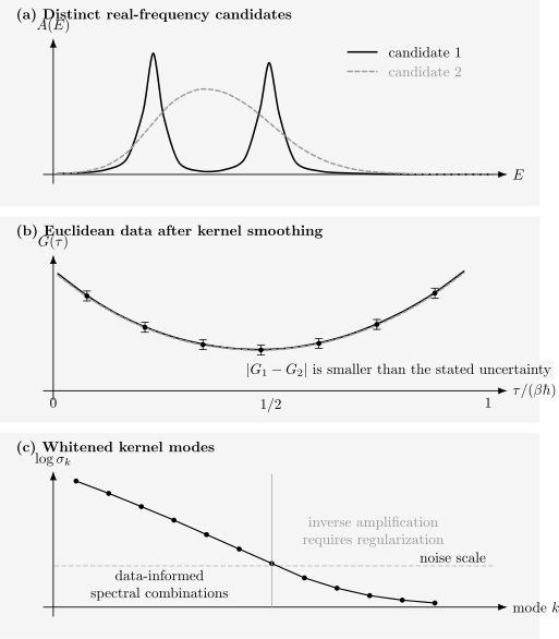
Kernel smoothing can map a resolved doublet and a broad band to Euclidean data that differ by less than the stated covariance. In the whitened singular basis, only modes with sufficiently large $\sigma_k$ are data informed; inversion of smaller modes amplifies uncertainty. A continuation should report the resulting ambiguity rather than selecting one detailed curve without qualification.

Truncated singular-value inversion

A truncated estimator keeps only modes above a chosen cutoff:

$$\mathbf a_r = \sum_{k=1}^{r} \frac{ \mathbf u_k^\dagger \widetilde{\mathbf g} }{ \sigma_k } \mathbf v_k.$$

This is stable after truncation, but it returns a projection of the spectrum onto the retained right-singular subspace. Changing $r$ changes the estimator’s resolution.

Tikhonov filtering

For quadratic regularization,

$$\mathbf a_\lambda = \underset{\mathbf a}{\operatorname{argmin}} \left[ \left\| \widetilde{\mathbf g} -\widetilde K\mathbf a \right\|_2^2 + \lambda \left\| L \left( \mathbf a-\mathbf a_0 \right) \right\|_2^2 \right].$$

When $L=I$ and $\mathbf a_0=0$,

$$\mathbf a_\lambda = \sum_k \frac{ \sigma_k }{ \sigma_k^2+\lambda } \left( \mathbf u_k^\dagger \widetilde{\mathbf g} \right) \mathbf v_k.$$

The filter factor

$$f_k(\lambda) = \frac{\sigma_k^2}{ \sigma_k^2+\lambda }$$

suppresses poorly constrained modes continuously. Stability is purchased by bias.

Resolution matrix

For the same quadratic case, the noise-free expectation satisfies

$$\mathbb E[ \mathbf a_\lambda ] = R_\lambda\mathbf a_{\mathrm{true}},$$

where

$$R_\lambda = V \operatorname{diag} \left( f_k(\lambda) \right) V^\dagger.$$

A row of $R_\lambda$ is a discrete resolution kernel. It shows how a nominal output energy mixes weight from neighboring energies. Reporting this kernel is more informative than quoting the spacing of the output grid.

Ill-Posed Does Not Mean Meaningless

In Hadamard’s terminology, a well-posed inverse problem has:

1. a solution;
2. a unique solution;
3. continuous dependence on the data.

Finite-data analytic continuation can violate uniqueness and continuous dependence in a broad spectral class. Regularization defines a nearby, stable estimation problem. It does not convert the original unrestricted inverse into a well-posed measurement of every spectral detail.

Useful information can still be robust:

• total spectral weight;
• low-order moments;
• a broad gap interval;
• the presence of weight in a large energy window;
• the position of an isolated dominant feature;
• a static susceptibility;
• a coarse transport scale.

The right question is often narrower than “reconstruct the entire spectrum.”

Regularization as Additional Information

A broad class of estimators minimizes

$$\Phi[\rho] = \frac12\chi^2[\rho] +\lambda\mathcal R[\rho],$$

subject to physical constraints. The regularizer $\mathcal R$ may encode:

• smoothness;
• proximity to a default model;
• sparsity in a chosen basis;
• few poles or bands;
• bounded variation;
• positivity;
• known support.

In Bayesian language,

$$p(\rho|\mathbf g) \propto p(\mathbf g|\rho) p(\rho),$$

where the likelihood contains the covariance and the prior contains assumptions about admissible spectra. Penalized optimization and Bayesian inference need not be identical, but both make the same conceptual point: finite data alone do not select a detailed spectrum.

Regularization is not an embarrassment to conceal. It is information to declare and test.

Physical Constraints

Constraints can remove unphysical candidates and improve precision. They cannot generate data resolution that is absent.

Positivity

For a normalized diagonal fermionic spectral function,

$$A(E)\geq0.$$

For a dynamic structure factor in a conjugate channel,

$$S(E)\geq0.$$

But ordinary positivity is not universal:

• a bosonic commutator spectrum changes sign across $E=0$;
• off-diagonal spectral components can be signed or complex;
• anomalous Green functions are not positive scalar measures;
• self-energy spectra require their own convention and analytic conditions.

Applying a positive-spectrum algorithm to a signed channel silently changes the inference problem.

Normalization and moments

Exact equal-time algebra can determine

$$M_n = \int dE\,E^n\rho(E).$$

Moments can be imposed as exact constraints only when they are genuinely exact in the same convention and numerical representation. If a moment comes from another uncertain calculation, it belongs in the likelihood with its covariance.

High-order moments emphasize spectral tails and can be numerically fragile. An inaccurate “exact” moment can force compensating artifacts elsewhere.

Support

Known lower or upper spectral bounds can be powerful. A guessed plotting window is not a physical support theorem. If appreciable weight lies outside the chosen window, normalization and moments can push that missing weight into false edge peaks.

Symmetry and detailed balance

Hermiticity, particle–hole symmetry, and KMS detailed balance can relate positive and negative energies. They should be enforced only when the operator, state, and convention possess the claimed symmetry.

For an ordered equilibrium spectrum,

$$S_{BA}(-E) = e^{-\beta E} S_{AB}(E).$$

This reduces redundant degrees of freedom, but it does not fix the line shape on the independent half-axis.

Causality and analytic structure

A physical retarded Green function is analytic in the upper half-plane. Its real and imaginary parts obey dispersion relations after any required subtractions. For positive scalar spectral measures, the corresponding Cauchy transform also has a definite half-plane sign.

Causality constraints reject some spurious rational functions and matrix continuations. They still leave a family of functions consistent with finite data.

Matrix positivity

For a matrix-valued fermionic spectrum,

$$A(E) = A^\dagger(E),$$

and

$$\mathbf x^\dagger A(E) \mathbf x \geq0$$

for every vector $\mathbf x$ in a positive spectral channel.

Continuing each matrix element independently can violate Hermiticity or positive semidefiniteness even when every diagonal entry looks reasonable. Matrix-aware parameterizations preserve the joint constraint.

Static and contact terms

Separate any known:

• equal-time discontinuity;
• delta function in time;
• frequency-independent offset;
• conserved bosonic zero mode;
• diamagnetic or contact contribution.

The dynamic spectral kernel should not be asked to mimic algebraic pieces it does not represent.

Choosing the Target

Before selecting an algorithm, write down:

1. the operator pair and ordering;
2. the thermal generator;
3. the imaginary-time or Matsubara transform;
4. the spectral density being inferred;
5. the relation between that density and the retarded observable;
6. all static and contact terms;
7. valid positivity, symmetry, support, and moment constraints.

For conductivity, for example, continuing a paramagnetic current correlator is not yet the full optical response. Diamagnetic terms, zero-frequency distributions, volume normalization, and limiting prescriptions must be handled through the Kubo Formula and the relevant transport convention.

Method Families

No continuation family is uniformly best. Each selects or averages over the admissible set differently.

• Rational or Padé: adds a low-order rational form and can excel for high-precision meromorphic data, but is vulnerable to noise-sensitive pole–zero artifacts.
• Maximum entropy: favors a positive spectrum near a default model and stably recovers broad structure, but smooths and biases according to the prior.
• Stochastic continuation: samples or optimizes constrained spectra and can expose nonparametric ambiguity, but its ensemble depends on the parameterization and sampling rule.
• Sparse or parametric: assumes few components in a chosen representation and can be highly interpretable when the model is valid, but can become overconfident under model mismatch.
• Nevanlinna or related interpolation: enforces half-plane analytic structure and preserves causality or positivity in the applicable class, but finite uncertain data still leave nonuniqueness.
• Direct real-axis or real-time methods: avoid Euclidean inversion for a target observable, while introducing separate finite-time, broadening, truncation, or solver errors.

Rational and Padé continuation

A rational approximant writes

$$\mathcal G(z) \approx \frac{ P_L(z) }{ Q_M(z) },$$

where $P_L$ and $Q_M$ are polynomials chosen to interpolate or fit the imaginary-axis data. Continued fractions are a common numerical representation.

This approach can be effective when:

• the input has very high precision;
• the analytic function is well represented by a modest number of poles;
• the frequency range is controlled;
• large-$z$ asymptotics are built in;
• the result is stable under precision, order, and point-selection changes.

It is fragile because nearby poles and zeros can cancel on the imaginary axis while producing large real-axis excursions. Noise may split one physical feature into several pole–zero pairs or place poles in the wrong half-plane.

A rational continuation should report:

• numerator and denominator orders;
• arithmetic precision;
• input points and weighting;
• pole locations and residues;
• near-canceling pole–zero pairs;
• stability across admissible orders;
• causality and sum-rule checks.

Smoothing the returned curve after a noisy Padé fit can hide unstable poles without repairing the inference.

Maximum-entropy spectral continuation

For a positive scalar spectrum $A(E)$ and positive default model $m(E)$, a common entropy is

$$S[A|m] = \int dE\, \left[ A(E)-m(E) -A(E) \ln \frac{A(E)}{m(E)} \right].$$

It satisfies

$$S[A|m]\leq0,$$

with equality at $A=m$. A maximum-entropy estimator balances fit and relative entropy:

$$Q[A] = \alpha S[A|m] -\frac12\chi^2[A].$$

The default model can encode known support, normalization scale, and coarse prior shape. The hyperparameter $\alpha$ controls how strongly departures from it are penalized.

There are several nonequivalent prescriptions for handling $\alpha$:

• maximize or average over an evidence approximation;
• use a discrepancy criterion for $\chi^2$;
• cross-validate held-out input modes;
• average over a declared hyperprior.

The output is conditional on this choice. A responsible analysis varies:

• the default-model shape;
• its normalization when not fixed;
• the frequency window;
• the output grid;
• the $\alpha$ prescription;
• the covariance treatment.

Maximum entropy is naturally formulated for positive measures. Signed spectra can sometimes be decomposed or reparameterized, but the result is a different prior problem and should not be presented as ordinary positive MaxEnt.

This spectral entropy is a regularizer over candidate functions. It is not the von Neumann entropy of a quantum state and does not follow directly from thermodynamic entropy maximization.

Stochastic analytic continuation

Stochastic methods represent the spectrum by movable peaks, bins, rectangles, basis coefficients, or other positive components and then sample or optimize configurations according to a data-fit and regularization rule.

A schematic sampling weight is

$$\mathcal P[A] \propto \exp \left[ -\frac{ \chi^2[A] }{ 2\Theta } \right] \mathcal P_0[A],$$

where $\Theta$ is an algorithmic sampling temperature or regularization control and $\mathcal P_0$ represents the measure over parameterized spectra.

Advantages include:

• nonparametric movement of spectral weight;
• straightforward positivity and normalization constraints;
• access to distributions of coarse features;
• less commitment to one smooth central solution.

Important limitations remain:

• a “uniform” measure depends on the parameterization;
• the sampling temperature is not automatically a physical temperature;
• the spread of sampled curves is not automatically a calibrated posterior interval;
• averaging can broaden peaks even when each sampled spectrum is sharp;
• optimization can lock onto spurious structure as the fit is tightened.

Report distributions of feature functionals, such as peak weight or gap edge, rather than using only the pointwise mean spectrum.

Sparse and parametric continuation

Suppose

$$\rho(E) = \sum_{r=1}^{p} \theta_r\phi_r(E),$$

where $\phi_r$ are chosen basis functions. Sparsity penalties, low-rank models, a few Lorentzians, pole expansions, known thresholds, and self-energy ansätze all restrict the candidate class.

Such models can give excellent resolution when the restriction is physically correct. They also make the conclusion conditional:

• a two-peak fit can resolve a doublet because it assumes a two-component family;
• a sparse pole basis favors isolated lines over continua;
• a smooth spline basis disfavors sharp thresholds;
• a Lorentzian model encodes a specific line shape and tail.

Model checks should include:

• comparison with less restrictive alternatives;
• residual structure in the whitened basis;
• parameter identifiability and correlations;
• synthetic tests with model mismatch;
• evidence or predictive performance where meaningful.

Machine-learned continuation belongs in the same category unless the training distribution is broad enough to define a defensible prior for the physical problem. A network cannot infer features absent from both the input information and its training assumptions.

Nevanlinna and causality-preserving interpolation

For a positive scalar spectral measure, the Cauchy transform belongs, up to convention-dependent signs, to a Herglotz–Nevanlinna class: it maps one half-plane into a definite half-plane and obeys strong analytic constraints.

Nevanlinna continuation uses this structure to parameterize all analytic interpolants consistent with exact input values and positivity. Continued-fraction or Schur-type constructions can preserve:

• analyticity;
• the correct half-plane sign;
• nonnegative normalized spectral weight in the applicable channel.

This is a major advantage over unconstrained rational interpolation. Its scope is still bounded:

• noisy data may need projection onto a feasible interpolation set;
• finite data leave a family of admissible analytic functions;
• a selection or averaging rule within that family adds assumptions;
• signed, anomalous, or matrix channels require appropriate generalizations;
• positivity and causality do not guarantee fine-feature identifiability.

Use the exact analytic class as a constraint, not as a promise of unlimited resolution.

Matrix-valued continuation

For orbital, spin, Nambu, or cluster Green functions, the target is a matrix function. Continuing matrix elements separately neglects their shared spectral geometry.

Safer approaches parameterize:

$$A(E) = B(E)B^\dagger(E)$$

in positive matrix channels, or continue quadratic forms

$$A_{\mathbf x}(E) = \mathbf x^\dagger A(E)\mathbf x$$

with consistency across a spanning set of vectors. Matrix maximum-entropy, Carathéodory, and related constructions are designed to preserve joint positivity and analyticity.

Basis covariance also matters. A method should transform consistently under a unitary change of orbital basis. Elementwise priors often do not.

Direct alternatives

When the scientific target is real frequency, it may be better to avoid Euclidean inversion:

• real-time tensor-network evolution;
• correction-vector or resolvent solvers;
• real-axis diagrammatic equations;
• Chebyshev or kernel-polynomial expansions;
• exact diagonalization with controlled finite-size broadening;
• nonequilibrium contour methods;
• experimentally forward-modeled response.

These methods have their own limits. A finite time $T$ gives a characteristic energy resolution

$$\Delta E \sim \frac{2\pi\hbar}{T},$$

and a resolvent evaluated at $E+i\eta$ returns an $\eta$-broadened spectrum. Avoiding analytic continuation exchanges one error structure for another; it does not remove the need for resolution analysis.

Ask Well-Posed Questions

Often the desired quantity is a linear spectral functional

$$Q[\rho] = \int dE\, q(E)\rho(E),$$

rather than every value of $\rho(E)$. Seek coefficients $w_i$ such that

$$q(E) \approx \sum_i w_iK_i(E).$$

Then

$$\widehat Q = \sum_iw_ig_i$$

estimates the functional directly. Its variance is

$$\operatorname{Var}(\widehat Q) = \mathbf w^\dagger C\mathbf w,$$

and its bias is controlled by the kernel mismatch

$$r(E) = q(E) -\sum_iw_iK_i(E).$$

This route can estimate a broad integrated weight or moment much more reliably than reconstructing a fine spectrum first and integrating the reconstruction afterward.

Examples of comparatively well-posed questions include:

• total weight in a wide energy interval;
• a low-order moment;
• a broad centroid;
• whether weight below a coarse threshold exceeds a bound;
• a smooth transport integral.

A narrow linewidth or sub-resolution doublet is usually a harder functional.

Worked Example: One Exact Pole

Consider

$$A(E) = Z\delta(E-E_0), \qquad Z>0.$$

Its Matsubara Green function is

$$\mathcal G(i\nu_n) = \frac{Z}{i\nu_n-E_0}.$$

If this one-pole form is known exactly, two generic exact complex data values can determine $Z$ and $E_0$. For example,

$$\frac{1}{ \mathcal G(i\nu_n) } = \frac{i\nu_n}{Z} -\frac{E_0}{Z}.$$

The reciprocal data lie on an affine function of $i\nu_n$.

This is not unrestricted analytic continuation. It is parameter estimation inside a two-parameter model. The apparent high resolution comes from the correct pole assumption.

If the true spectrum contains a continuum,

$$A(E) = Z\delta(E-E_0) +A_{\mathrm{inc}}(E),$$

the same fit can absorb continuum effects into biased $Z$ and $E_0$. Residuals, model expansion, and synthetic mismatch tests are therefore essential.

Worked Example: An Unresolved Doublet

Take two equal lines centered at $E_0$:

$$A_\Delta(E) = \frac{Z}{2} \left[ \delta \left( E-E_0-\frac{\Delta}{2} \right) + \delta \left( E-E_0+\frac{\Delta}{2} \right) \right].$$

For a smooth kernel,

$$G_\Delta = \frac{Z}{2} \left[ K \left( E_0+\frac{\Delta}{2} \right) + K \left( E_0-\frac{\Delta}{2} \right) \right].$$

Expanding around $E_0$ gives

$$G_\Delta = ZK(E_0) + \frac{ Z\Delta^2 }{8} K''(E_0) +O(\Delta^4).$$

The linear term cancels. Sensitivity to a small symmetric splitting begins at order $\Delta^2$. If

$$\left\| \frac{ Z\Delta^2 }{8} C^{-1/2} K''(E_0) \right\|_2 \lesssim1,$$

the doublet is not distinguished from a single line at the covariance scale. A method may still draw two peaks because its model or prior prefers them, but the input has not independently resolved the splitting.

Worked Example: Static Bosonic Weight

Let $Q$ be conserved:

$$[Q,\mathcal K]=0.$$

For $\delta Q=Q-\langle Q\rangle$,

$$C_{QQ}(\tau) = \left\langle (\delta Q)^2 \right\rangle$$

is constant, and

$$C_{QQ}(i\Omega_\ell) = \beta \operatorname{Var}(Q) \delta_{\ell0}.$$

The commutator spectrum vanishes because $[Q(t),Q]=0$. A continuation of only the regular commutator kernel cannot recover this constant term. If the zero-frequency datum is included without a separate static component, the optimizer may invent arbitrarily narrow low-energy weight.

This is a representation error, not merely poor regularization.

From Spectrum to Retarded Response

The continuation endpoint should be a causal quantity with a declared prescription:

$$\mathcal G^{\mathrm R}(E) = \int dE'\, \frac{\rho(E')}{E-E'+i0^+}.$$

In numerical plots, one often uses

$$\mathcal G_\eta^{\mathrm R}(E) = \int dE'\, \frac{\rho(E')}{E-E'+i\eta}, \qquad \eta>0.$$

Its imaginary part is a Lorentzian convolution:

$$-\frac1\pi \operatorname{Im} \mathcal G_\eta^{\mathrm R}(E) = \int dE'\, \frac1\pi \frac{\eta}{ (E-E')^2+\eta^2 } \rho(E').$$

The display broadening $\eta$ must not be confused with:

• intrinsic decay width;
• continuation resolution;
• finite-size level spacing;
• experimental energy resolution.

All four can broaden a plotted feature, but they have different meanings.

Data Preparation

Continuation cannot repair an inconsistent input correlator.

Equilibrate and estimate autocorrelation

For Monte Carlo data, verify equilibration, block beyond the integrated autocorrelation scale, and propagate the same blocked samples into means and covariance. An underestimated covariance invites overfitting.

Enforce identities before fitting

Check:

• endpoint and parity relations;
• equal-time discontinuities;
• complex-conjugation symmetry;
• Matsubara positive-negative frequency pairing;
• known asymptotic tails;
• exact normalization;
• static zero-mode contributions.

If an identity is imposed by symmetrization, recompute the covariance after that linear transformation.

Avoid double counting

Imaginary-time data and Matsubara data obtained from the same samples are not independent. Fitting both with separate diagonal error bars double counts information unless their joint covariance is included.

Subtract known tails analytically

If

$$\mathcal G(i\nu) = \sum_{r=0}^{R} \frac{M_r}{(i\nu)^{r+1}} +\mathcal G_{\mathrm{rem}}(i\nu),$$

subtract the known asymptotic part and continue the better-conditioned remainder. Restore the tail afterward. This reduces dynamic range but does not remove the inverse problem.

Choose dimensionless variables

Rescale energy and amplitudes so the numerical problem has moderate magnitudes. Record the transformation so normalization, moments, and covariance are restored correctly.

A Credible Continuation Workflow

1. Define the scientific claim

State whether the target is:

• a full spectral density;
• a broad gap;
• one peak position;
• an integrated weight;
• a linewidth;
• a transport coefficient;
• a causal self-energy.

The harder the functional, the stronger the required resolution evidence.

2. Audit the forward convention

Derive the kernel from the declared correlator. Verify a free mode or exact finite-system benchmark, including signs, $\hbar$, temperature, and contact terms.

3. Preserve the statistical model

Carry the covariance, sample count, blocking procedure, and systematic solver errors. Whiten residuals and inspect them for structure.

4. Declare the admissible class

List:

• positivity or sign constraints;
• normalization and moments;
• support;
• symmetry and detailed balance;
• causality;
• static components;
• smoothness, sparsity, or parametric assumptions.

Separate exact constraints from modeling choices.

5. Calibrate with synthetic data

Generate spectra spanning plausible alternatives, apply the same grid and kernel, and add noise with the measured covariance:

$$\mathbf g_{\mathrm{syn}} = K\mathbf a_{\mathrm{syn}} +\boldsymbol\epsilon, \qquad \boldsymbol\epsilon \sim \mathcal N(0,C).$$

Then run the complete analysis without using the known answer. Include adversarial cases:

• one peak versus a close doublet;
• sharp threshold versus rounded onset;
• narrow peak plus broad background;
• missing support outside the fit window;
• a spectrum violating the chosen model family.

Synthetic success on only the same shapes favored by the prior is not a resolution test.

6. Perturb the analysis

Repeat under:

• bootstrap or jackknife resamples;
• removal of selected input points;
• modest covariance regularization changes;
• plausible default models;
• output-grid and window changes;
• regularization strengths;
• alternative algorithmic parameterizations.

Record which functionals remain stable.

7. Use predictive checks

Hold out selected imaginary-time points or whitened singular components, fit the remainder, and predict the held-out data. This tests interpolation in the data domain. It does not by itself prove real-axis uniqueness, because several spectra may share the same predictions.

8. Compare methods by shared claims

Agreement between methods is useful only when their assumptions differ meaningfully. Two codes using positive smoothness priors can agree because they encode similar bias.

Compare:

• forward residuals;
• exact constraints;
• broad integrated features;
• ambiguity under each method;
• synthetic resolution.

Do not demand pointwise agreement where the data do not support it.

9. Report an ambiguity set

When possible, identify spectra satisfying

$$\chi^2[\rho] \leq \chi^2_{\mathrm{acceptable}}$$

and all exact constraints. Extremize the scientific functional over this set:

$$Q_{\min} = \underset{\rho\in\mathcal A}{\inf} Q[\rho], \qquad Q_{\max} = \underset{\rho\in\mathcal A}{\sup} Q[\rho].$$

This turns “many spectra fit” into a quantitative interval for the claim of interest.

10. Separate resolution from visualization

Choose plotting broadening and interpolation only after the inferential resolution has been assessed. A dense, smooth frequency grid is a display choice.

Reporting Standard

A reproducible continuation result should state:

1. the operator and Green-function convention;
2. $\beta$, chemical potential, units, and kernel;
3. the input grid and number of independent samples;
4. the full covariance treatment;
5. contact, tail, and static-term preprocessing;
6. spectral window and discretization;
7. exact constraints and uncertain auxiliary constraints;
8. method, prior or regularizer, and hyperparameter rule;
9. arithmetic precision and convergence criteria;
10. synthetic-data resolution tests;
11. sensitivity to priors, points, grid, and window;
12. uncertainty on physically interpreted functionals;
13. any additional display broadening.

For a claimed doublet or linewidth, include the closest unresolved alternative that still fits the data. For a claimed gap, report the operational threshold and the smallest detectable in-gap weight.

Interpreting Uncertainty

Several uncertainties coexist:

• sampling uncertainty: finite stochastic or experimental samples;
• solver uncertainty: truncation, convergence, discretization, and finite size;
• kernel uncertainty: temperature, calibration, or forward-model parameters;
• regularization uncertainty: hyperparameter and prior choice;
• model uncertainty: whether the admissible spectral family is appropriate;
• non-identifiability: multiple admissible spectra predict indistinguishable data.

A narrow bootstrap band from one fixed regularizer captures only part of this list. In strongly ill-posed settings, model and non-identifiability uncertainty can dominate pointwise sampling uncertainty.

Common Mistakes

Treating substitution as an algorithm

Writing

$$i\zeta_\ell \mapsto E+i0^+$$

is valid after the analytic function has been identified. It does not specify how to reconstruct that function from a finite table.

Invoking the identity theorem on Matsubara points

The Matsubara grid has no finite accumulation point. Uniqueness requires the physical analytic and asymptotic class, not merely the statement that the function is analytic.

Ignoring covariance

Diagonal error bars can overcount heavily correlated time points and drive the reconstruction toward noise.

Forcing positivity in the wrong channel

Bosonic commutator spectra, off-diagonal matrix elements, anomalous functions, and many self-energy conventions are not ordinary nonnegative scalar measures.

Confusing fit quality with resolution

A very small $\chi^2$ may indicate overfitting. It does not prove that narrow structures are physical.

Reading grid spacing as energy resolution

An output grid spacing of $10^{-3}$ does not imply that features separated by $10^{-3}$ are identifiable. Resolution follows from the kernel, covariance, and assumptions.

Reporting only one default model

One smooth reconstruction conceals prior dependence. Vary the default over physically plausible alternatives while preserving exact constraints.

Treating stochastic spread as automatic error bars

The sampled ensemble depends on its measure, parameterization, and algorithmic temperature. Calibration requires synthetic and coverage tests.

Continuing matrix elements independently

Elementwise fits can violate Hermiticity, positive semidefiniteness, basis covariance, and common pole structure.

Hiding static weight in a narrow peak

A conserved bosonic contribution belongs to a separate zero Matsubara term. Represent it explicitly.

Overinterpreting cross-method agreement

Methods with similar positivity and smoothness assumptions can return similar curves from the same underdetermined data.

Broadening twice

Continuation regularization, finite-time windows, resolvent $\eta$, and plotting convolution can all broaden structure. Track each operation separately.

Calling a prior a theorem

Smoothness, sparsity, few-pole structure, and default models can be physically motivated. They remain assumptions unless derived for the system and observable.

Practical Checklist

Before accepting a real-frequency claim, ask:

1. Is the exact forward kernel correct for the channel?
2. Are contact and static terms separate?
3. Is the covariance propagated and numerically credible?
4. Which constraints are exact, and which are priors?
5. Does the output obey causality, symmetry, normalization, and moments?
6. What singular or resolution modes are data informed?
7. Which alternative spectra fit within the same uncertainty?
8. Has the full workflow passed synthetic model-mismatch tests?
9. Is the interpreted feature stable under point, prior, grid, and window changes?
10. Would a direct spectral functional answer the scientific question more robustly?
11. Is display broadening reported separately?
12. Are conclusions phrased at the demonstrated resolution?

Connections

• The exact forward kernels, thermal weights, and zero-mode decomposition are derived in Spectral Representation.
• The discrete frequency grids and zero-frequency bookkeeping are fixed in Bosonic and Fermionic Matsubara Frequencies.
• Causality, upper-half-plane analyticity, and dispersion relations are developed in Retarded and Advanced Response.
• Physical peak, continuum, residue, and linewidth interpretation belongs to Spectral Functions.
• DMFT for Quantum Materials owns the material loop and the decision to continue specified Green functions, self-energies, or response objects; this page retains the covariance, resolution, regularization, and ambiguity audit for every real-frequency claim.
• Exact moment constraints and their operator origins belong to Sum Rules.
• Ordered observable spectra and detailed balance are related to response through the Fluctuation–Dissipation Theorem.
• Static susceptibilities can often be obtained without reconstructing a full dynamic spectrum; see Susceptibilities.
• Transport continuation requires contact terms and limit ordering from Transport Coefficients Preview.

References

• G. Baym and N. D. Mermin, “Determination of Thermodynamic Green’s Functions,” Journal of Mathematical Physics 2, 232–234 (1961); uniqueness of the thermal continuation under the required analytic and asymptotic conditions.
• H. J. Vidberg and J. W. Serene, “Solving the Eliashberg Equations by Means of N-Point Padé Approximants,” Journal of Low Temperature Physics 29, 179–192 (1977); the classic rational-continuation construction.
• A. N. Tikhonov and V. Y. Arsenin, Solutions of Ill-Posed Problems, Winston, 1977; foundational regularization framework.
• M. Jarrell and J. E. Gubernatis, “Bayesian Inference and the Analytic Continuation of Imaginary-Time Quantum Monte Carlo Data,” Physics Reports 269, 133–195 (1996); detailed maximum-entropy review and covariance-aware formulation.
• A. W. Sandvik, “Stochastic Method for Analytic Continuation of Quantum Monte Carlo Data,” Physical Review B 57, 10287–10290 (1998); stochastic spectral sampling and diagnostics for spurious structure.
• O. Gunnarsson, M. W. Haverkort, and G. Sangiovanni, “Analytical Continuation of Imaginary Axis Data Using Maximum Entropy,” Physical Review B 81, 155107 (2010); statistical and default-model contributions to continuation error.
• D. Bergeron and A.-M. S. Tremblay, “Algorithms for Optimized Maximum Entropy and Diagnostic Tools for Analytic Continuation,” Physical Review E 94, 023303 (2016); implementation, hyperparameter, and diagnostic analysis.
• O. Goulko, A. S. Mishchenko, L. Pollet, N. Prokof’ev, and B. Svistunov, “Numerical Analytic Continuation: Answers to Well-Posed Questions,” Physical Review B 95, 014102 (2017); ambiguity-aware inference for feature-level questions.
• G. J. Kraberger, R. Triebl, M. Zingl, and M. Aichhorn, “Maximum Entropy Formalism for the Analytic Continuation of Matrix-Valued Green’s Functions,” Physical Review B 96, 155128 (2017); signed off-diagonal components and joint matrix constraints.
• J. Fei, C.-N. Yeh, and E. Gull, “Nevanlinna Analytical Continuation,” Physical Review Letters 126, 056402 (2021); causality- and positivity-preserving interpolation in the applicable Green-function class.
• J. Fei, C.-N. Yeh, D. Zgid, and E. Gull, “Analytical Continuation of Matrix-Valued Functions: Carathéodory Formalism,” Physical Review B 104, 165111 (2021); analytic continuation that preserves matrix-valued positivity structure.

Exercises

1. Finite interpolation is not uniqueness

Let $z_1,\ldots,z_N$ be distinct points in the upper half-plane, and suppose $F(z)$ is analytic there. Construct a nonzero analytic perturbation $h(z)$ that vanishes at every $z_j$ and decays as $1/z$ for large $z$ within the upper half-plane. What does this prove, and what does it not prove, about thermal Green functions?

Solution

Choose $\Lambda>0$ and define

$$h(z) = \epsilon \frac{ \displaystyle \prod_{j=1}^{N} (z-z_j) }{ (z+i\Lambda)^{N+1} }.$$

The only pole is at $z=-i\Lambda$, which lies in the lower half-plane. Thus $h$ is analytic in the upper half-plane. At every input point,

$$h(z_j)=0.$$

For large $z$ in the upper half-plane,

$$h(z) \sim \frac{\epsilon}{z}.$$

Therefore $F(z)$ and $F(z)+h(z)$ agree at all $N$ sampled points but differ elsewhere.

This proves that finitely many interpolation conditions do not determine an arbitrary upper-half-plane analytic function. It does not prove that both candidates are physical Green functions. The perturbation may violate positivity, reflection properties, moments, or the joint upper- and lower-half-plane spectral representation. Baym–Mermin uniqueness concerns infinitely many exact thermal samples inside the proper physical class.

2. Quantify singular-mode noise amplification

A whitened kernel has two singular values

$$\sigma_1=1, \qquad \sigma_2=10^{-4}.$$

Suppose the whitened data error has magnitude $10^{-2}$ along each left singular vector.

1. Find the formal inverse error along each right singular vector.
2. For Tikhonov regularization with $L=I$ and $\lambda=10^{-4}$, find the resolution filter factors $f_k$.

Solution

Formal inversion divides a data-mode error by the corresponding singular value:

$$\delta c_k = \frac{ \delta\widetilde g_k }{ \sigma_k }.$$

Thus

$$\delta c_1 = 10^{-2},$$

while

$$\delta c_2 = \frac{10^{-2}}{10^{-4}} = 10^2.$$

The second spectral component is effectively unconstrained by a unit-scale prior.

The Tikhonov resolution factors are

$$f_k = \frac{ \sigma_k^2 }{ \sigma_k^2+\lambda }.$$

Therefore

$$f_1 = \frac{1}{1+10^{-4}} \approx 0.9999,$$

and

$$f_2 = \frac{10^{-8}}{10^{-8}+10^{-4}} \approx 10^{-4}.$$

The well-measured mode is nearly retained, whereas the unstable mode is almost completely suppressed. The stable output is correspondingly biased toward the retained subspace.

3. Correlated data do not count twice

Two estimates $g_1$ and $g_2$ have equal variance $\sigma^2$ and correlation coefficient $r$:

$$C = \sigma^2 \begin{pmatrix} 1&r\\ r&1 \end{pmatrix}.$$

For the average

$$\bar g = \frac{g_1+g_2}{2},$$

find its variance. Compare it with the variance inferred by incorrectly treating the points as independent. Evaluate the ratio for $r=0.9$.

Solution

Write

$$\mathbf w = \frac12 \begin{pmatrix} 1\\ 1 \end{pmatrix}.$$

Then

$$\begin{aligned} \operatorname{Var}(\bar g) &= \mathbf w^{\mathsf T} C \mathbf w \\ &= \frac{\sigma^2}{2} (1+r). \end{aligned}$$

If the points were independent, one would report

$$\operatorname{Var}_{\mathrm{diag}}(\bar g) = \frac{\sigma^2}{2}.$$

The true variance is larger by the factor

$$\frac{ \operatorname{Var}(\bar g) }{ \operatorname{Var}_{\mathrm{diag}}(\bar g) } = 1+r.$$

For $r=0.9$, the factor is $1.9$. Two strongly correlated points contain much less than twice the information of one point.

4. Derive the doublet sensitivity

For

$$A_\Delta(E) = \frac{Z}{2} \left[ \delta \left( E-E_0-\frac{\Delta}{2} \right) + \delta \left( E-E_0+\frac{\Delta}{2} \right) \right],$$

show that the difference from a single line $Z\delta(E-E_0)$ begins at order $\Delta^2$ for any smooth forward kernel $K(E)$.

Solution

The doublet prediction is

$$G_\Delta = \frac{Z}{2} \left[ K \left( E_0+\frac{\Delta}{2} \right) + K \left( E_0-\frac{\Delta}{2} \right) \right].$$

Taylor expansion gives

$$\begin{aligned} K \left( E_0\pm\frac{\Delta}{2} \right) ={}& K(E_0) \pm \frac{\Delta}{2} K'(E_0) \\ &+ \frac{\Delta^2}{8} K''(E_0) +O(\Delta^3). \end{aligned}$$

Adding the two expansions cancels all odd terms:

$$G_\Delta = ZK(E_0) + \frac{ Z\Delta^2 }{8} K''(E_0) +O(\Delta^4).$$

The single-line prediction is $G_0=ZK(E_0)$. Hence

$$G_\Delta-G_0 = \frac{ Z\Delta^2 }{8} K''(E_0) +O(\Delta^4).$$

This quadratic suppression explains why close symmetric doublets are difficult to resolve.

5. Check the positivity class

A Hermitian bosonic operator in a two-level system has commutator spectral density

$$\rho(E) = w \left[ \delta(E-\Delta) -\delta(E+\Delta) \right], \qquad w>0, \quad \Delta>0.$$

Is $\rho(E)$ a nonnegative measure? Verify the correct sign condition and explain why ordinary positive MaxEnt is inappropriate without reparameterization.

Solution

At positive energy the line has weight $+w$, whereas at negative energy it has weight $-w$. Thus $\rho$ is not a nonnegative measure.

Multiplication by $E$ gives positive weight at both lines:

$$\begin{aligned} E\rho(E) ={}& w\Delta\delta(E-\Delta) \\ &+ w\Delta\delta(E+\Delta). \end{aligned}$$

Therefore

$$E\rho(E)\geq0$$

as a distribution. A positive-spectrum entropy applied directly to $\rho$ would forbid the required negative-energy line and change the physical channel. One may instead infer a positive ordered spectrum on an independent half-axis and impose detailed balance, or use a signed-spectrum formulation derived for the chosen convention.

6. Derive a MaxEnt stationarity equation

Discretize a positive spectrum as components $a_j>0$ with default components $m_j>0$. Let

$$S(\mathbf a|\mathbf m) = \sum_j \left[ a_j-m_j -a_j\ln \frac{a_j}{m_j} \right],$$

and

$$Q(\mathbf a) = \alpha S -\frac12 \left\| \widetilde{\mathbf g} -\widetilde K\mathbf a \right\|_2^2.$$

Find the stationarity equation for an interior maximum.

Solution

The entropy derivative is

$$\frac{\partial S}{\partial a_j} = -\ln \frac{a_j}{m_j}.$$

The misfit derivative is

$$\frac{\partial}{\partial\mathbf a} \left[ -\frac12 \left\| \widetilde{\mathbf g} -\widetilde K\mathbf a \right\|_2^2 \right] = \widetilde K^\dagger \left( \widetilde{\mathbf g} -\widetilde K\mathbf a \right).$$

Setting the total derivative to zero gives

$$\alpha \ln \frac{a_j}{m_j} = \left[ \widetilde K^\dagger \left( \widetilde{\mathbf g} -\widetilde K\mathbf a \right) \right]_j.$$

Equivalently,

$$a_j = m_j \exp \left\{ \frac1\alpha \left[ \widetilde K^\dagger \left( \widetilde{\mathbf g} -\widetilde K\mathbf a \right) \right]_j \right\}.$$

The equation is nonlinear because $\mathbf a$ appears in the residual. It also makes the default-model role explicit: when the data gradient is weak relative to $\alpha$, $a_j$ remains near $m_j$.

7. Estimate a spectral functional directly

In a discretized problem,

$$\mathbf g = K\mathbf a +\boldsymbol\epsilon, \qquad \mathbb E[ \boldsymbol\epsilon ]=0, \qquad \mathbb E[ \boldsymbol\epsilon \boldsymbol\epsilon^\dagger ]=C.$$

The target is

$$Q = \mathbf q^\dagger\mathbf a.$$

Among linear estimators $\widehat Q=\mathbf w^\dagger\mathbf g$ that are unbiased for every $\mathbf a$, derive the minimum-variance weights. Assume the required inverses exist.

Solution

Unbiasedness for every $\mathbf a$ requires

$$K^\dagger\mathbf w = \mathbf q.$$

The variance is

$$\operatorname{Var}(\widehat Q) = \mathbf w^\dagger C\mathbf w.$$

Introduce a multiplier vector $\boldsymbol\lambda$ and minimize

$$\mathcal L = \mathbf w^\dagger C\mathbf w -2\operatorname{Re} \left[ \boldsymbol\lambda^\dagger \left( K^\dagger\mathbf w-\mathbf q \right) \right].$$

Stationarity with respect to $\mathbf w^\dagger$ gives

$$C\mathbf w = K\boldsymbol\lambda.$$

Thus

$$\mathbf w = C^{-1}K\boldsymbol\lambda.$$

Imposing unbiasedness yields

$$K^\dagger C^{-1} K \boldsymbol\lambda = \mathbf q.$$

Therefore

$$\mathbf w = C^{-1} K \left( K^\dagger C^{-1} K \right)^{-1} \mathbf q.$$

The minimum variance is

$$\operatorname{Var}(\widehat Q) = \mathbf q^\dagger \left( K^\dagger C^{-1} K \right)^{-1} \mathbf q.$$

If the inverse does not exist or the variance is enormous, exact unbiased estimation of that functional is unavailable. One can then trade controlled bias for lower variance by approximating $\mathbf q$ in the row space of $K$.

8. Separate a conserved zero mode

Suppose the measured bosonic correlator is

$$C(i\Omega_\ell) = \beta V\delta_{\ell0} + \int dE\, \frac{ \rho(E) }{ i\Omega_\ell-E },$$

with $V\geq0$. Explain how you would prepare these data for continuation and give two failures caused by omitting the first term.

Solution

Represent $V$ as a separate static parameter. If it is known independently, subtract

$$\beta V\delta_{\ell0}$$

before fitting the dynamical kernel. If it is uncertain, fit it jointly with $\rho$ using its prior information or covariance, while keeping it algebraically distinct.

Omitting the static term can cause:

1. a spurious very narrow peak near $E=0$ as the dynamical spectrum attempts to reproduce the excess zero-frequency datum;
2. distortion of broad low-energy weight or the inferred gap because normalization and regularization redistribute the unmatched static contribution.

Dropping the $\ell=0$ datum without explanation avoids one mismatch but discards information about $V$ and may conceal a physically important conserved fluctuation.