Retarded and Advanced Response

A retarded response function answers an operational question: how does an observable measured at time $t$ change when a weak source acts at an earlier time $t'$? Its advanced partner uses the opposite support condition. The advanced function is not an instruction for an experiment to respond before it is perturbed. It is the adjoint boundary value needed to state spectral, analytic, and reciprocity identities cleanly.

For a perturbation

$$H_{\mathrm{pert}}(t) = -f(t)B,$$

the convention used here is

$$\chi^{\mathrm R}_{AB}(t) = \frac{i}{\hbar} \theta(t) \left\langle [A(t),B(0)] \right\rangle,$$

where $A$ is the detector and $B$ is the operator coupled to the source. The advanced partner is

$$\chi^{\mathrm A}_{AB}(t) = -\frac{i}{\hbar} \theta(-t) \left\langle [A(t),B(0)] \right\rangle.$$

The two functions contain the same commutator spectrum but approach it from opposite sides of the real-frequency axis. That pairing is the organizing idea of this page.

Canonical Scope

This page is the canonical home for the retarded–advanced pair as many-body response functions. It owns:

• two-time retarded and advanced commutator definitions;
• temporal support and the precise meaning of causality;
• adjoint, Hermitian-conjugation, and frequency-reflection identities;
• upper- and lower-half-plane analyticity;
• retarded and advanced Lehmann boundary values;
• the response spectral density as their discontinuity;
• reactive and absorptive parts;
• Kramers–Kronig and subtracted dispersion relations;
• pole, cut, damping, and stability diagnostics;
• exact oscillator and two-level benchmarks;
• numerical checks that use the pair together.

Neighboring pages retain separate ownership:

• Kubo Formula derives the response from a source-coupled density operator and owns contact terms, static limits, conductivity, and material applications.
• Retarded and Advanced Green Functions owns inverse kernels of Schrödinger-type operators and their boundary prescriptions.
• Green Functions in Many-Body QM owns normal single-particle propagators, including fermionic anticommutator functions and $N\pm1$ spectra.
• Time-Dependent Correlations owns ordinary ordered correlators, dephasing, recurrence, and finite-time spectra.
• Structure Factors owns scattering spectra rather than causal response.
• Fluctuations and Susceptibilities owns equilibrium thermodynamic derivatives and Kubo–Mori covariance.
• Susceptibilities owns named magnetic, density, compressibility, and pairing channels, their units, and measurement protocols.
• Spectral Functions owns line-shape interpretation, quasiparticle and resonance criteria, linewidths, and experimental convolution.
• Fluctuation–Dissipation Theorem owns KMS detailed balance and the equilibrium conversion between response and fluctuations.
• Spectral Representation owns the exact thermal bridge from Lehmann weights and Matsubara data to retarded boundary values, including static bosonic terms.
• Analytic Continuation owns numerical reconstruction from finite uncertain imaginary-axis data.
• Sum Rules owns the full nested-commutator and high-energy moment hierarchy. Transport coefficients remain in the following treatment.

Real-Time Thermal Dynamics Preview explains when retarded response is sufficient and when initial-state, lesser, and closed-time-path data are additionally required. Relativistic microcausality, renormalized field-theory response, and reusable analytic-continuation algorithms lie beyond this boundary.

Convention Ledger

Response signs cannot be checked by memory alone. They must be traced through the source coupling, operator order, and Fourier transform.

Source convention

The perturbation is

$$H_{\mathrm{pert}}(t) = -f(t)B.$$

With this minus sign, the first-order response of $A$ uses

$$+\frac{i}{\hbar} \left\langle [A(t),B(t')] \right\rangle.$$

If the perturbation is instead written $H_{\mathrm{pert}}=+fB$, the susceptibility entering the response law changes sign. A paper that defines a retarded Green function with $-i\theta\langle[A,B]\rangle$ may still be physically consistent; its source-response relation can contain an additional minus sign.

Fourier convention

For a stationary kernel,

$$\chi(\omega) = \int_{-\infty}^{\infty} dt\, e^{i\omega t} \chi(t),$$

with inverse

$$\chi(t) = \int_{-\infty}^{\infty} \frac{d\omega}{2\pi}\, e^{-i\omega t} \chi(\omega).$$

Thus a real harmonic source is represented through components proportional to $e^{-i\omega t}$. Retarded functions are analytic for $\operatorname{Im}z\gt0$ and carry $+i0$ in denominators of the form $\hbar\omega-\Delta E+i0$.

The variable $\omega$ is angular frequency. If energy $E=\hbar\omega$ is used instead, the Fourier measure and delta functions acquire the corresponding factors of $\hbar$.

Reference state

The expectation value is taken in an unperturbed state $\rho_0$:

$$\langle X\rangle_0 = \operatorname{Tr}(\rho_0X).$$

The two-time definitions require no equilibrium assumption. Stationarity,

$$[H_0,\rho_0]=0,$$

is needed before reducing the dependence from $(t,t')$ to $t-t'$ and introducing one frequency.

Operator labels

The order $\chi_{AB}$ means response of detector $A$ to a source coupled through $B$. In general,

$$\chi_{AB} \ne \chi_{BA}.$$

The operators need not be Hermitian. Adjoint relations must therefore retain daggers until a Hermitian channel basis has been specified.

Two-Time Definitions

In the Heisenberg picture of the unperturbed Hamiltonian, define

$$\begin{aligned} \chi^{\mathrm R}_{AB}(t,t') ={}& \frac{i}{\hbar} \theta(t-t') \\ &\times \operatorname{Tr} \left\{ \rho_0 [A_H(t),B_H(t')] \right\}, \end{aligned}$$

and

$$\begin{aligned} \chi^{\mathrm A}_{AB}(t,t') ={}& -\frac{i}{\hbar} \theta(t'-t) \\ &\times \operatorname{Tr} \left\{ \rho_0 [A_H(t),B_H(t')] \right\}. \end{aligned}$$

Their support is opposite:

$$\chi^{\mathrm R}_{AB}(t,t') =0 \qquad \text{for }t\lt t',$$

while

$$\chi^{\mathrm A}_{AB}(t,t') =0 \qquad \text{for }t\gt t'.$$

Away from coincident times,

$$\begin{aligned} \chi^{\mathrm R}_{AB}(t,t') - \chi^{\mathrm A}_{AB}(t,t') ={}& \frac{i}{\hbar} \\ &\times \left\langle [A_H(t),B_H(t')] \right\rangle_0. \end{aligned}$$

The pair therefore splits the full commutator into its future- and past-supported parts.

Coincident-time convention

For nonsingular operators, changing $\theta(0)$ alters a function at one point and does not affect ordinary time integrals. Equal-time distributions, canonical commutators, derivatives of step functions, and explicitly source-dependent observables can generate contact terms for which this shorthand is insufficient.

The response must then be treated distributionally. Kubo Formula owns the source derivative and contact-term bookkeeping.

What Causality Means

The retarded support condition says that a source insertion at $t'$ does not change the detector expectation value at an earlier time $t$. For a source history,

$$\delta\langle A(t)\rangle = \int_{-\infty}^{\infty} dt'\, \chi^{\mathrm R}_{AB}(t,t') f(t'),$$

only $t'\le t$ contributes.

This is temporal causality of a response protocol. It does not by itself imply:

• a relativistic light cone;
• finite propagation speed in nonrelativistic continuum mechanics;
• exponential decay in space;
• irreversibility of the closed microscopic dynamics;
• validity of a Markov approximation.

Nonrelativistic Hamiltonians can have unbounded group velocities, and spatial kernels can develop tails immediately while remaining exactly retarded in time. Causality, Support, and Interpretation in Nonrelativistic QM owns that distinction.

Nonstationary states

For a quench, driven state, or aging system,

$$\chi^{\mathrm R}(t,t') \ne \chi^{\mathrm R}(t-t')$$

in general. The support condition remains meaningful, but a one-variable $\chi(\omega)$ does not. A Wigner transform can introduce average and relative times,

$$T=\frac{t+t'}{2}, \qquad \tau=t-t',$$

but then $\chi(T,\omega)$ is a time-local spectral representation, not an equilibrium susceptibility. Gradient expansions require an additional separation of time scales.

Why the Advanced Function Matters

The advanced function is not normally the kernel used for an initial-value experiment. It is nevertheless indispensable because it:

1. is the adjoint boundary value of the retarded response;
2. isolates the spectral discontinuity $\chi^{\mathrm R}-\chi^{\mathrm A}$;
3. separates reactive and absorptive matrix parts;
4. supplies consistency checks for numerical calculations;
5. appears naturally in final-value problems and products of retarded and advanced propagators;
6. identifies which complex-frequency singularities are compatible with stability.

Calling $\chi^{\mathrm A}$ “acausal” without qualification is therefore misleading. It has past support as a Green-function boundary condition. It does not assert that the physical retarded experiment depends on future source values.

Adjoint Identities

The identity

$$\langle X\rangle_0^* = \langle X^\dagger\rangle_0$$

gives

$$\begin{aligned} \left[ \chi^{\mathrm R}_{AB}(t,t') \right]^* ={}& \chi^{\mathrm A}_{B^\dagger A^\dagger} (t',t). \end{aligned}$$

This relation uses only Hermiticity of the density operator and the definitions above. It does not require thermal equilibrium or time-reversal symmetry.

For a stationary state, write $\tau=t-t'$. Then

$$\left[ \chi^{\mathrm R}_{AB}(\tau) \right]^* = \chi^{\mathrm A}_{B^\dagger A^\dagger} (-\tau).$$

At real frequency,

$$\left[ \chi^{\mathrm R}_{AB}(\omega) \right]^* = \chi^{\mathrm A}_{B^\dagger A^\dagger} (\omega).$$

Matrix response

Choose Hermitian channel operators $A_a=A_a^\dagger$. The response matrices obey

$$\boldsymbol{\chi}^{\mathrm A}(\omega) = \boldsymbol{\chi}^{\mathrm R}(\omega)^\dagger.$$

Thus define the Hermitian reactive and absorptive matrices

$$\boldsymbol{\chi}'(\omega) = \frac{1}{2} \left[ \boldsymbol{\chi}^{\mathrm R}(\omega) + \boldsymbol{\chi}^{\mathrm A}(\omega) \right],$$

and

$$\boldsymbol{\chi}''(\omega) = \frac{1}{2i} \left[ \boldsymbol{\chi}^{\mathrm R}(\omega) - \boldsymbol{\chi}^{\mathrm A}(\omega) \right].$$

For one Hermitian autocorrelation channel, these reduce to the ordinary real and imaginary parts of $\chi^{\mathrm R}$.

Frequency reflection

For a Hermitian autocorrelation channel, $\chi^{\mathrm R}_{AA}(t)$ is real. Therefore

$$\chi^{\mathrm R}_{AA}(-\omega) = \left[ \chi^{\mathrm R}_{AA}(\omega) \right]^*.$$

Consequently,

$$\operatorname{Re}\chi^{\mathrm R}_{AA}(-\omega) = \operatorname{Re}\chi^{\mathrm R}_{AA}(\omega),$$

and

$$\operatorname{Im}\chi^{\mathrm R}_{AA}(-\omega) = -\operatorname{Im}\chi^{\mathrm R}_{AA}(\omega).$$

These parity statements do not apply component by component to an arbitrary non-Hermitian cross-susceptibility.

Response Spectral Density

For a stationary state, define the commutator spectral density

$$\begin{aligned} \rho_{AB}(\omega) ={}& \frac{1}{2\pi\hbar} \int_{-\infty}^{\infty} dt\, e^{i\omega t} \\ &\times \left\langle [A(t),B(0)] \right\rangle_0. \end{aligned}$$

With this normalization,

$$\chi^{\mathrm R}_{AB}(\omega) - \chi^{\mathrm A}_{AB}(\omega) = 2\pi i\, \rho_{AB}(\omega).$$

For a Hermitian channel matrix,

$$\boldsymbol{\chi}''(\omega) = \pi\boldsymbol{\rho}(\omega).$$

The response spectral density is not the same object as an ordinary positive correlation spectrum. It is a population-weighted difference of the two operator orders. At thermal equilibrium, that difference is what distinguishes absorption from stimulated emission.

Lehmann Representation

Let

$$H_0\lvert n\rangle = E_n\lvert n\rangle, \qquad \rho_0 = \sum_n p_n \lvert n\rangle\langle n\rvert.$$

Define

$$A_{nm} = \langle n\lvert A\rvert m\rangle, \qquad B_{mn} = \langle m\lvert B\rvert n\rangle.$$

The spectral density is

$$\begin{aligned} \rho_{AB}(\omega) ={}& \frac{1}{\hbar} \sum_{n,m} (p_n-p_m) A_{nm}B_{mn} \\ &\times \delta\!\left( \omega-\frac{E_m-E_n}{\hbar} \right). \end{aligned}$$

The retarded boundary value is

$$\chi^{\mathrm R}_{AB}(\omega) = \sum_{n,m} \frac{ (p_m-p_n)A_{nm}B_{mn} }{ \hbar\omega+E_n-E_m+i0 },$$

while the advanced boundary value is

$$\chi^{\mathrm A}_{AB}(\omega) = \sum_{n,m} \frac{ (p_m-p_n)A_{nm}B_{mn} }{ \hbar\omega+E_n-E_m-i0 }.$$

The numerator and the pole prescription play different roles:

• $E_m-E_n$ fixes transition frequencies;
• $A_{nm}B_{mn}$ fixes source and detector visibility;
• $p_n-p_m$ fixes the population imbalance;
• $\pm i0$ fixes temporal support.

Replacing $i0$ by a finite width is an additional physical, limiting, or numerical assumption. It is not part of the exact finite-system Lehmann formula.

Passive equilibrium and positive frequency

For $A=B=A^\dagger$ in a Gibbs state, an upward transition with $E_m\gt E_n$ has

$$p_n-p_m\gt0.$$

Therefore

$$\rho_{AA}(\omega)\ge0 \qquad \text{for }\omega\gt0,$$

and, with the present sign convention,

$$\operatorname{Im} \chi^{\mathrm R}_{AA}(\omega) \ge0 \qquad \text{for }\omega\gt0.$$

A generic cross-susceptibility has no componentwise positivity. In a matrix of Hermitian source channels, positivity applies to the absorptive quadratic form for physically allowed positive-frequency source combinations in a passive state.

Population inversion can reverse the sign. Negative absorption then indicates gain rather than an algebraic inconsistency.

Analyticity from Support

For complex frequency

$$z=x+iy,$$

the retarded transform is

$$\chi^{\mathrm R}(z) = \int_0^\infty dt\, e^{izt} \chi^{\mathrm R}(t).$$

If $y\gt0$, then

$$\lvert e^{izt}\rvert = e^{-yt},$$

which damps the large-$t$ integrand. Under the usual integrability or tempered-distribution conditions, $\chi^{\mathrm R}(z)$ is analytic in the upper half-plane.

Similarly,

$$\chi^{\mathrm A}(z) = \int_{-\infty}^0 dt\, e^{izt} \chi^{\mathrm A}(t)$$

is analytic for $\operatorname{Im}z\lt0$.

Causal support implies the corresponding analyticity. The converse requires suitable growth and boundary-value assumptions; an arbitrary analytic function is not automatically a physical response.

Boundary values

The physical frequency functions are limits:

$$\chi^{\mathrm R}(\omega) = \lim_{\eta\to0^+} \chi(\omega+i\eta),$$

and

$$\chi^{\mathrm A}(\omega) = \lim_{\eta\to0^+} \chi(\omega-i\eta).$$

The signs follow from the chosen $e^{+i\omega t}$ transform. Reversing the Fourier sign reverses the half-plane bookkeeping.

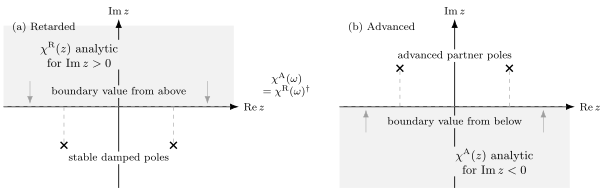
With the $e^{+i\omega t}$ transform, $\chi^{\mathrm R}$ is analytic for $\operatorname{Im}z>0$ and is approached from above; a stable damped retarded pole lies below the real axis. The advanced partner has the reflected structure. Exact isolated finite-system poles are recovered as the damping tends to zero and the poles approach the real axis with opposite $i0$ prescriptions.

Poles, Cuts, and Stability

An exact finite isolated system has a discrete Lehmann spectrum. Its frequency-domain response is a sum of real-axis poles interpreted as distributions with $\pm i0$ boundary values.

Several limits change that structure:

• a thermodynamic limit can turn dense poles into branch cuts;
• coupling to a continuum can move resonance poles away from the real axis on an analytically continued sheet;
• an open-system or phenomenological equation can produce finite damping directly;
• finite observation time broadens spectral resolution without creating an intrinsic lifetime.

For a stable retarded response, poles of a damped effective model lie in the lower half-plane. A pole

$$z_\star = \Omega-i\Gamma, \qquad \Gamma\gt0,$$

contributes

$$e^{-iz_\star t} = e^{-i\Omega t}e^{-\Gamma t}$$

for $t\gt0$. A pole in the upper half-plane instead produces exponential growth and signals an instability, an active medium, or an inconsistent approximation.

The advanced partner has reflected poles in the upper half-plane because it is supported for negative time. This reflection is not a physical instability of the retarded experiment.

Spectral Representation

For $\operatorname{Im}z\ne0$ and sufficient high-frequency decay,

$$\chi_{AB}(z) = \int_{-\infty}^{\infty} d\omega'\, \frac{ \rho_{AB}(\omega') }{ \omega'-z }.$$

Approaching the real axis from above gives

$$\begin{aligned} \chi^{\mathrm R}_{AB}(\omega) ={}& \operatorname{PV} \int_{-\infty}^{\infty} d\omega'\, \frac{ \rho_{AB}(\omega') }{ \omega'-\omega } \\ &+ i\pi\rho_{AB}(\omega), \end{aligned}$$

whereas approaching from below gives

$$\begin{aligned} \chi^{\mathrm A}_{AB}(\omega) ={}& \operatorname{PV} \int_{-\infty}^{\infty} d\omega'\, \frac{ \rho_{AB}(\omega') }{ \omega'-\omega } \\ &- i\pi\rho_{AB}(\omega). \end{aligned}$$

The principal-value part is shared. The on-shell discontinuity changes sign.

This representation makes the advanced function useful even when only retarded response is measured: together they separate the dispersive and absorptive information without ambiguity.

Dispersion Relations

For a scalar Hermitian channel with adequate decay,

$$\operatorname{Re} \chi^{\mathrm R}(\omega) = \frac{1}{\pi} \operatorname{PV} \int_{-\infty}^{\infty} d\omega'\, \frac{ \operatorname{Im}\chi^{\mathrm R}(\omega') }{ \omega'-\omega }.$$

The companion relation is

$$\operatorname{Im} \chi^{\mathrm R}(\omega) = -\frac{1}{\pi} \operatorname{PV} \int_{-\infty}^{\infty} d\omega'\, \frac{ \operatorname{Re}\chi^{\mathrm R}(\omega') }{ \omega'-\omega }.$$

For matrices, replace ordinary real and imaginary parts by $\boldsymbol{\chi}'$ and $\boldsymbol{\chi}''$:

$$\boldsymbol{\chi}'(\omega) = \frac{1}{\pi} \operatorname{PV} \int_{-\infty}^{\infty} d\omega'\, \frac{ \boldsymbol{\chi}''(\omega') }{ \omega'-\omega }.$$

These Kramers–Kronig relations are consequences of support, analyticity, and high-frequency control. They are not an independent microscopic law.

Subtractions and contact terms

If $\chi(z)$ approaches a nonzero constant or grows at high frequency, an unsubtracted dispersion integral does not converge. Apply the relation to the decaying part or use a subtraction:

$$\begin{aligned} \chi(z)-\chi(z_0) ={}& (z-z_0) \int_{-\infty}^{\infty} d\omega'\, \\ &\times \frac{ \rho(\omega') }{ (\omega'-z)(\omega'-z_0) }. \end{aligned}$$

Instantaneous source derivatives can contribute polynomial or constant terms that are not reconstructed from the absorptive commutator spectrum alone. Conductivity is a standard example because the physical current may contain a diamagnetic contact term.

Finite bandwidth

Experimental and numerical data cover a finite frequency window. A direct Hilbert transform then misses spectral weight outside the window and can generate edge artifacts. Reliable checks require:

• an explicit high-frequency tail model or bound;
• subtraction constants fixed independently;
• uncertainty propagation;
• window sensitivity tests;
• exact moment constraints where available.

A visually smooth Kramers–Kronig transform is not by itself evidence that the underlying response is causal.

High-Frequency Expansion

Expanding the spectral representation for large $z$ gives

$$\chi_{AB}(z) = -\frac{1}{z} \int d\omega'\, \rho_{AB}(\omega') - \frac{1}{z^2} \int d\omega'\, \omega'\rho_{AB}(\omega') + \cdots.$$

The zeroth moment is

$$\int_{-\infty}^{\infty} d\omega\, \rho_{AB}(\omega) = \frac{1}{\hbar} \langle[A,B]\rangle_0.$$

For $A=B$, the equal-time commutator vanishes, so a regular autocorrelation susceptibility often begins at order $1/z^2$. Derivatives, conserved currents, unbounded operators, and contact terms require domain care.

The systematic nested-commutator hierarchy belongs to Sum Rules.

Impulse and Harmonic Response

For a stationary kernel,

$$\delta\langle A(t)\rangle = \int_{-\infty}^{\infty} dt'\, \chi^{\mathrm R}_{AB}(t-t') f(t').$$

An impulsive source

$$f(t)=f_0\delta(t)$$

gives

$$\delta\langle A(t)\rangle = f_0\chi^{\mathrm R}_{AB}(t),$$

so the retarded kernel is literally the impulse response.

For a monochromatic component

$$f(t)=f_0e^{-i\omega t},$$

the steady linear response is

$$\delta\langle A(t)\rangle = \chi^{\mathrm R}_{AB}(\omega) f_0e^{-i\omega t}.$$

For a scalar channel, $\operatorname{Re}\chi^{\mathrm R}$ controls the in-phase reactive response and $\operatorname{Im}\chi^{\mathrm R}$ controls the quadrature component. With a passive diagonal channel and the source convention used here, the cycle-averaged absorbed power is nonnegative at positive frequency.

Exact Harmonic-Oscillator Benchmark

Consider

$$H_0 = \frac{p^2}{2m} + \frac{1}{2}m\omega_0^2x^2$$

and a force coupling

$$H_{\mathrm{pert}}(t) = -f(t)x.$$

The Heisenberg commutator is state independent:

$$[x(t),x(0)] = -\frac{i\hbar}{m\omega_0} \sin(\omega_0t).$$

Therefore

$$\chi^{\mathrm R}_{xx}(t) = \frac{\theta(t)}{m\omega_0} \sin(\omega_0t),$$

and

$$\chi^{\mathrm A}_{xx}(t) = -\frac{\theta(-t)}{m\omega_0} \sin(\omega_0t).$$

The frequency-domain pair is

$$\chi^{\mathrm R}_{xx}(\omega) = \frac{1}{ m\left[ \omega_0^2-(\omega+i0)^2 \right] },$$

and

$$\chi^{\mathrm A}_{xx}(\omega) = \frac{1}{ m\left[ \omega_0^2-(\omega-i0)^2 \right] }.$$

For real $\omega$,

$$\chi^{\mathrm A}_{xx}(\omega) = \left[ \chi^{\mathrm R}_{xx}(\omega) \right]^*.$$

The positive-frequency absorptive part is

$$\operatorname{Im} \chi^{\mathrm R}_{xx}(\omega) = \frac{\pi}{2m\omega_0} \delta(\omega-\omega_0) \qquad (\omega\gt0).$$

The exact isolated oscillator has a delta line, not a finite linewidth.

Effective damping

A phenomenological damped equation,

$$m\ddot x + m\gamma\dot x + m\omega_0^2x = f,$$

has

$$\chi^{\mathrm R}_{\mathrm{damp}}(\omega) = \frac{1}{ m\left( \omega_0^2-\omega^2-i\gamma\omega \right) }.$$

For $\gamma\gt0$, its retarded poles lie below the real axis. The advanced partner changes $-i\gamma\omega$ to $+i\gamma\omega$. This finite width models coupling, coarse graining, or an effective bath; it is not obtained by merely renaming the exact $i0$.

Two-Level Benchmark

Let

$$H_0 = \frac{\hbar\Omega}{2}\sigma_z,$$

and couple a source through $B=\sigma_x$, with detector $A=\sigma_x$. If

$$p_g-p_e = \Delta p,$$

then

$$\chi^{\mathrm R}_{xx}(t) = \frac{2\Delta p}{\hbar} \theta(t) \sin(\Omega t).$$

Its frequency representation is

$$\begin{aligned} \chi^{\mathrm R}_{xx}(\omega) ={}& \frac{\Delta p}{\hbar} \left[ \frac{1}{\omega+\Omega+i0} \right. \\ &\left. - \frac{1}{\omega-\Omega+i0} \right]. \end{aligned}$$

At positive temperature, $\Delta p\gt0$, so the line at $\omega=\Omega$ has positive absorptive weight. For an inverted population, $\Delta p\lt0$ and the same transition provides gain.

This example separates three facts that are often conflated:

• the transition frequency comes from $H_0$;
• the line weight comes from the matrix element and population difference;
• the retarded pole side comes from causality.

Reciprocity Is an Additional Symmetry

The adjoint identity

$$\boldsymbol{\chi}^{\mathrm A} = \boldsymbol{\chi}^{\mathrm R\dagger}$$

follows from the definitions. Onsager–Casimir reciprocity requires more: equilibrium, microscopic reversibility, a correctly transformed external magnetic field $\mathcal B$, and operators with definite time-reversal parities $\epsilon_A$ and $\epsilon_B$.

Under those assumptions, a common response convention gives

$$\chi^{\mathrm R}_{AB} (\omega;\mathcal B) = \epsilon_A\epsilon_B \chi^{\mathrm R}_{BA} (\omega;-\mathcal B).$$

The exact component form depends on whether spatial momenta, currents, pseudovectors, and complex channel bases are present. Reversing operator labels without also reversing time-reversal-odd control parameters is not a valid reciprocity test.

Time Reversal owns the antiunitary transformation rules. Static Maxwell reciprocity of equilibrium derivatives is a related but distinct statement.

Conserved Quantities and Static Limits

If $B$ commutes with the unperturbed Hamiltonian,

$$[B,H_0]=0,$$

then $B(t)=B$. For the diagonal channel,

$$\chi^{\mathrm R}_{BB}(t)=0$$

because $[B,B]=0$.

The thermodynamic derivative

$$\left. \frac{\partial\langle B\rangle_f} {\partial f} \right|_{f=0}$$

can nevertheless be nonzero because an equilibrating bath reweights sectors with different $B$. There is no contradiction: isolated real-time response and equilibrium state comparison are different protocols.

Likewise,

$$\lim_{\mathbf q\to0} \lim_{\omega\to0} \chi(\mathbf q,\omega)$$

need not equal

$$\lim_{\omega\to0} \lim_{\mathbf q\to0} \chi(\mathbf q,\omega).$$

The Kubo Formula owns these order-of-limits questions in depth.

Relation to Other Two-Point Functions

The same operators can define several inequivalent objects:

Object	Ordering or support	Main role
$\langle A(t)B(0)\rangle$	ordinary order	transition and fluctuation spectrum
$\frac12\langle\{A(t),B(0)\}\rangle$	symmetrized	noise-like fluctuations
$\chi^{\mathrm R}_{AB}$	commutator, future support	physical causal response
$\chi^{\mathrm A}_{AB}$	commutator, past support	adjoint boundary value
time-ordered correlator	chronological order	perturbation theory
Matsubara correlator	imaginary-time order	equilibrium thermal calculations

Equilibrium relations can reconstruct one object from another only after specifying temperature, statistics, operator order, and analytic continuation. The Fluctuation–Dissipation Relation owns the thermal conversion between fluctuation spectra and absorptive response.

Numerical Evaluation

Exact diagonalization

For a finite Hilbert space, the Lehmann sum is direct. A robust implementation should:

1. diagonalize $H_0$ and normalize the probabilities $p_n$;
2. compute source and detector matrix elements independently;
3. retain the population difference $p_n-p_m$;
4. build retarded and advanced denominators with opposite signs;
5. verify the adjoint relation;
6. compare integrated spectral moments with equal-time commutators.

A Lorentzian display replaces

$$\delta(\omega-\omega_{mn})$$

by a normalized kernel of width $\eta$. The resulting smooth curve depends on $\eta$ and should not be reported as an intrinsic decay rate unless a controlled continuum or bath calculation supplies that interpretation.

Real-time evolution

One may compute the commutator in time and multiply by the appropriate step function. A finite record of duration $T$ gives resolution

$$\Delta\omega \sim \frac{2\pi}{T}.$$

Windowing reduces ringing but convolves the spectrum with the window transform. Compute retarded and advanced functions from the same commutator data so that their discontinuity and adjoint relation remain controlled.

Analytic continuation

At equilibrium, a bosonic Matsubara susceptibility samples an analytic function on imaginary frequencies. The formal continuation is

$$i\nu_n \longrightarrow \omega+i0.$$

Spectral Representation derives this exact equilibrium bridge and fixes its sign conventions. Reconstructing real-frequency data from finitely many noisy imaginary-axis samples is ill conditioned. Causality, positivity where applicable, moments, and asymptotic behavior are constraints, not a guarantee of a unique stable spectrum. Analytic Continuation develops the corresponding regularized inverse problem and resolution tests.

Experimental Interpretation

A phase-resolved driven experiment can determine the complex retarded susceptibility by comparing the amplitude and phase of the response to the source. The advanced response is generally not measured by arranging a detector to react before the drive. Instead, it is inferred as the adjoint boundary value when the assumptions behind

$$\boldsymbol{\chi}^{\mathrm A} = \boldsymbol{\chi}^{\mathrm R\dagger}$$

hold.

Different probes access different source–detector pairs. Magnetic resonance, density modulation, optical conductivity, neutron scattering, and pump–probe spectroscopy should not be assigned the same $\chi_{AB}$ without writing their coupling Hamiltonians and detector observables.

Validation Checklist

Before trusting a retarded-response calculation, verify:

1. the perturbation sign and coupled operator;
2. the detector–source order in $\chi_{AB}$;
3. retarded support in time;
4. upper-half-plane analyticity for the chosen Fourier sign;
5. $\chi^{\mathrm A}=\chi^{\mathrm R\dagger}$ in a Hermitian channel basis;
6. positive-frequency passivity for diagonal equilibrium channels;
7. Kramers–Kronig consistency with justified tails or subtractions;
8. exact equal-time and high-frequency moments;
9. finite-size and broadening dependence;
10. static, uniform, thermodynamic, and zero-damping orders of limits.

Common Mistakes

• Calling an ordinary correlation spectrum a retarded susceptibility.
• Using an anticommutator for an observable Kubo response merely because the microscopic particles are fermions.
• Treating the advanced kernel as evidence of backward-in-time signaling.
• Forgetting to transpose source and detector labels in the adjoint relation.
• Pairing the $e^{+i\omega t}$ transform with the wrong half-plane.
• Replacing $i0$ by a finite linewidth without naming the physical or numerical origin.
• Assuming every cross-susceptibility has a positive imaginary part.
• Applying unsubtracted Kramers–Kronig relations to a response with a contact term.
• Inferring a lifetime from finite-window broadening.
• Equating an isolated zero-frequency retarded response with an isothermal derivative.
• Claiming Onsager reciprocity without checking time-reversal parities and external fields.

Reliable Workflow

1. Write $H_{\mathrm{pert}}$ and identify $A$ and $B$.
2. Fix the Fourier transform and frequency units.
3. Decide whether the reference state is stationary.
4. Compute the full commutator or its Lehmann weights.
5. Apply future support for $\chi^{\mathrm R}$ and past support for $\chi^{\mathrm A}$.
6. Verify the adjoint relation before interpreting spectra.
7. Separate reactive, absorptive, and contact contributions.
8. Test analyticity, dispersion relations, moments, and passivity.
9. Repeat across broadening, size, time-window, and order-of-limits choices.
10. Report which features are exact, limiting, phenomenological, or resolution induced.

Exercises

Exercise 1: Support and analyticity

Suppose $\chi^{\mathrm R}(t)$ vanishes for $t\lt0$ and obeys

$$\int_0^\infty dt\, e^{-\eta t} \lvert\chi^{\mathrm R}(t)\rvert \lt\infty$$

for every $\eta\gt0$. Show that its Fourier–Laplace transform is analytic for $\operatorname{Im}z\gt0$.

Solution

Write

$$\chi^{\mathrm R}(z) = \int_0^\infty dt\, e^{izt} \chi^{\mathrm R}(t).$$

For $z=x+iy$ with $y\gt0$,

$$\lvert e^{izt}\rvert=e^{-yt}.$$

The assumed bound therefore gives absolute convergence on every closed strip $y\ge\eta\gt0$. Differentiation under the integral is allowed there:

$$\frac{d\chi^{\mathrm R}}{dz} = i \int_0^\infty dt\, t e^{izt} \chi^{\mathrm R}(t),$$

provided the corresponding exponentially weighted first moment is finite; more generally one uses standard dominated-convergence arguments locally in the upper half-plane. Hence the transform is complex differentiable and analytic for $\operatorname{Im}z\gt0$.

The support condition alone does not determine the growth class. That is why the integrability or tempered-distribution qualification matters.

Exercise 2: Adjoint relation

Starting from the two-time definitions, prove

$$\left[ \chi^{\mathrm R}_{AB}(t,t') \right]^* = \chi^{\mathrm A}_{B^\dagger A^\dagger}(t',t).$$

Solution

Complex conjugation gives

$$\begin{aligned} \left[ \chi^{\mathrm R}_{AB}(t,t') \right]^* ={}& -\frac{i}{\hbar} \theta(t-t') \\ &\times \left\langle [A(t),B(t')]^\dagger \right\rangle. \end{aligned}$$

The adjoint of the commutator is

$$[A(t),B(t')]^\dagger = [B^\dagger(t'),A^\dagger(t)].$$

The same step function is precisely the past-support factor for an advanced kernel whose first time argument is $t'$ and whose second time argument is $t$. The result is therefore

$$\begin{aligned} \chi^{\mathrm A}_{B^\dagger A^\dagger}(t',t) ={}& -\frac{i}{\hbar} \theta(t-t') \\ &\times \left\langle [B^\dagger(t'),A^\dagger(t)] \right\rangle. \end{aligned}$$

Exercise 3: Oscillator pair

Use

$$[x(t),x(0)] = -\frac{i\hbar}{m\omega_0} \sin(\omega_0t)$$

to derive $\chi^{\mathrm R}_{xx}(t)$, $\chi^{\mathrm A}_{xx}(t)$, and their frequency-domain forms.

Solution

Multiplying the commutator by the two support factors gives

$$\chi^{\mathrm R}_{xx}(t) = \frac{\theta(t)}{m\omega_0} \sin(\omega_0t),$$

and

$$\chi^{\mathrm A}_{xx}(t) = -\frac{\theta(-t)}{m\omega_0} \sin(\omega_0t).$$

For the retarded transform, include $e^{-\eta t}$ with $\eta\gt0$:

$$\begin{aligned} \chi^{\mathrm R}_{xx}(\omega) ={}& \frac{1}{m\omega_0} \int_0^\infty dt\, e^{i\omega t-\eta t} \sin(\omega_0t) \\ ={}& \frac{1}{ m\left[ \omega_0^2-(\omega+i\eta)^2 \right] }. \end{aligned}$$

Taking $\eta\to0^+$ yields the retarded expression. The negative-time integral gives

$$\chi^{\mathrm A}_{xx}(\omega) = \frac{1}{ m\left[ \omega_0^2-(\omega-i0)^2 \right] }.$$

For real frequency the two are complex conjugates.

Exercise 4: Two-level absorption and inversion

For the two-level benchmark, show that the positive-frequency absorptive line changes sign when the populations are inverted.

Solution

The positive-frequency pole is

$$-\frac{\Delta p}{\hbar} \frac{1}{\omega-\Omega+i0}.$$

Using

$$\operatorname{Im} \frac{1}{x+i0} = -\pi\delta(x),$$

gives

$$\operatorname{Im} \chi^{\mathrm R}_{xx}(\omega) = \frac{\pi\Delta p}{\hbar} \delta(\omega-\Omega)$$

at $\omega\gt0$. In a passive state, $\Delta p=p_g-p_e\gt0$, so the line absorbs. Under inversion, $\Delta p\lt0$, and the line has negative absorptive weight, corresponding to gain.

The pole location is unchanged. Inversion changes the residue, not the transition energy or retarded boundary prescription.

Exercise 5: Discontinuity and dispersion

Assume

$$\chi(z) = \int d\omega'\, \frac{\rho(\omega')}{\omega'-z}.$$

Derive the retarded–advanced discontinuity and the first Kramers–Kronig relation.

Solution

The distribution identities are

$$\frac{1}{x-i0} = \operatorname{PV}\frac{1}{x} + i\pi\delta(x),$$

and

$$\frac{1}{x+i0} = \operatorname{PV}\frac{1}{x} - i\pi\delta(x).$$

For $x=\omega'-\omega$, the retarded boundary approaches $z=\omega+i0$, so its denominator is $x-i0$:

$$\chi^{\mathrm R}(\omega) = \operatorname{PV} \int d\omega'\, \frac{\rho(\omega')}{\omega'-\omega} + i\pi\rho(\omega).$$

The advanced boundary has the opposite sign. Therefore

$$\chi^{\mathrm R}(\omega) - \chi^{\mathrm A}(\omega) = 2\pi i\rho(\omega).$$

For a scalar Hermitian channel,

$$\rho(\omega) = \frac{1}{\pi} \operatorname{Im} \chi^{\mathrm R}(\omega).$$

Substitution into the shared principal-value part gives

$$\operatorname{Re} \chi^{\mathrm R}(\omega) = \frac{1}{\pi} \operatorname{PV} \int d\omega'\, \frac{ \operatorname{Im}\chi^{\mathrm R}(\omega') }{ \omega'-\omega }.$$

Exercise 6: Conserved observable

Let $[B,H_0]=0$. Explain why $\chi^{\mathrm R}_{BB}(t)=0$ but the isothermal susceptibility of $B$ can be nonzero.

Solution

Conservation gives

$$B(t)=B.$$

Hence

$$[B(t),B(0)] = [B,B] =0,$$

so the isolated retarded commutator vanishes.

An isothermal perturbation changes the equilibrium density operator:

$$\rho_f \propto e^{-\beta(H_0-fB)}.$$

It can therefore reweight sectors with different eigenvalues of $B$. When $B$ commutes with $H_0$,

$$\left. \frac{\partial\langle B\rangle_f} {\partial f} \right|_{f=0} = \beta\operatorname{Var}(B),$$

which need not vanish. The two quantities describe different protocols: isolated unitary response versus re-equilibration with a bath.

Exercise 7: Pole diagnosis

A proposed retarded susceptibility contains a pole at

$$z_\star = \Omega+i\Gamma, \qquad \Gamma\gt0.$$

What does this imply, and what checks should be made before calling the model unstable?

Solution

For the inverse transform at $t\gt0$, the pole contributes

$$e^{-iz_\star t} = e^{-i\Omega t}e^{+\Gamma t}.$$

The response grows exponentially, and the pole lies inside the half-plane where a stable retarded response should be analytic. This indicates an instability, gain, or an inconsistent approximation.

Before drawing a physical conclusion, check:

• the Fourier-transform sign;
• whether the object is retarded rather than advanced;
• the sign of the damping or self-energy convention;
• whether the expansion was made about an unstable reference state;
• whether a numerical analytic continuation reflected the pole incorrectly;
• whether the active drive genuinely supplies gain.

After those checks, an upper-half-plane retarded pole is a meaningful instability diagnostic.

Exercise 8: Cross-response positivity

Why does

$$\operatorname{Im} \chi^{\mathrm R}_{AA}(\omega)\ge0 \qquad (\omega\gt0)$$

for a passive Hermitian autocorrelation channel not imply

$$\operatorname{Im} \chi^{\mathrm R}_{AB}(\omega)\ge0$$

for every pair $A\ne B$?

Solution

For $A=A^\dagger$, the diagonal Lehmann residue contains

$$(p_n-p_m) \lvert A_{nm}\rvert^2,$$

which is nonnegative at positive frequency in a passive thermal state.

For a cross response, the residue is

$$(p_n-p_m) A_{nm}B_{mn}.$$

The product can be complex or have either sign. Positivity is instead a statement about the absorptive quadratic form of the full channel matrix for a physical source combination. Individual off-diagonal entries need not be positive.

Cross-Links

• Correlation Function Definitions — sign, source, Fourier-transform, and response-spectrum conventions.
• Linear Response Formula Sheet — compact Kubo, spectral, fluctuation, static-limit, and transport formulas.
• Kubo Formula — source derivation, contact terms, static limits, and applications.
• Susceptibilities — named response channels, units, tensors, and protocol choices.
• Green Functions in Many-Body QM — number-changing single-particle propagators.
• Spectral Functions — poles versus peaks, continua, linewidths, and forward-model interpretation.
• Fluctuation–Dissipation Theorem — equilibrium ordered, symmetrized, and absorptive spectral relations.
• Spectral Representation — thermal Lehmann weights, Matsubara transforms, analytic boundary values, and static bosonic terms.
• Sum Rules — exact response moments and large-complex-energy coefficients.
• Time-Dependent Correlations — ordinary correlators and finite-time spectra.
• Structure Factors — scattering spectra and detailed balance.
• Fluctuations and Susceptibilities — thermodynamic response and Kubo–Mori covariance.
• Retarded and Advanced Green Functions — inverse kernels and $i0$ boundary prescriptions.
• Green Functions and Response Preview — introductory response bridge.
• Spectral Representation of Green Functions — resolvent spectral theorem.
• Fluctuation–Dissipation Relation — equilibrium conversion between noise and absorption.
• Random Phase Approximation — approximate collective response and pole diagnostics.
• Time Reversal — antiunitary symmetry and parity conventions.
• Fourier Transform Conventions — transform signs and normalization.

References

1. R. Kubo, “Statistical-Mechanical Theory of Irreversible Processes. I”, Journal of the Physical Society of Japan 12, 570–586 (1957).
2. H. B. Callen and T. A. Welton, “Irreversibility and Generalized Noise”, Physical Review 83, 34–40 (1951).
3. L. Onsager, “Reciprocal Relations in Irreversible Processes. I”, Physical Review 37, 405–426 (1931).
4. L. Onsager, “Reciprocal Relations in Irreversible Processes. II”, Physical Review 38, 2265–2279 (1931).
5. H. B. G. Casimir, “On Onsager’s Principle of Microscopic Reversibility”, Reviews of Modern Physics 17, 343–350 (1945).
6. H. Lehmann, “Über Eigenschaften von Ausbreitungsfunktionen und Renormierungskonstanten quantisierter Felder”, Il Nuovo Cimento 11, 342–357 (1954).
7. R. Kubo, M. Toda, and N. Hashitsume, Statistical Physics II: Nonequilibrium Statistical Mechanics, 2nd ed., Springer, 1991.
8. G. D. Mahan, Many-Particle Physics, 3rd ed., Kluwer Academic/Plenum, 2000.
9. A. L. Fetter and J. D. Walecka, Quantum Theory of Many-Particle Systems, Dover, 2003.
10. D. Forster, Hydrodynamic Fluctuations, Broken Symmetry, and Correlation Functions, CRC Press, 1990.
11. H. Bruus and K. Flensberg, Many-Body Quantum Theory in Condensed Matter Physics, Oxford University Press, 2004.
12. N. W. Ashcroft and N. D. Mermin, Solid State Physics, Brooks/Cole, 1976.