Correlation Functions Overview

A many-body correlation function is an expectation value of an ordered product of operators at specified positions, times, or modes. Correlators answer targeted questions that a many-body wavefunction does not answer at a glance: whether distant regions fluctuate together, whether order persists, which momenta dominate, which excitation energies can be reached, how rapidly memory is lost, and how a system responds to a weak probe.

For a state $\rho$,

$$\langle X\rangle_\rho = \operatorname{Tr}(\rho X).$$

The basic two-point function is therefore

$$G_{AB}(1,2) = \left\langle A(1)B(2) \right\rangle_\rho,$$

where each label can include site, position, time, spin, orbital, or other indices. This compact notation is incomplete until the state, operator order, time prescription, normalization, and boundary conditions are stated.

Correlations are central in many-body physics because low-order local observables are often measurable and computationally accessible even when the full state occupies an exponentially large Hilbert space. They are not a magical compression of all information: a small set of low-order correlators generally does not determine an arbitrary interacting state.

Canonical Scope

This page is the canonical overview of correlation functions as many-body diagnostics. It organizes one-point, two-point, higher-point, connected, spatial, and temporal correlators; explains their decay and long-range limits; and distinguishes fluctuations, Green functions, response functions, and structure factors.

Detailed derivations remain in their focused homes:

• Correlations and Covariance owns covariance as a measurement statistic for observables.
• Correlation Functions in Path Integrals owns path-integral insertion formulas and source-based representations.
• Bath Correlation Functions owns environmental memory, noise spectra, and master-equation rates.
• Kubo Formula owns the generic many-body source-to-response derivation, Lehmann representation, contact terms, and transport limits.
• Interacting Systems and Approximation Methods routes from a declared model, target correlator, regime, and control parameter to an approximation family and its validation tests.
• Interacting Many-Body Systems Overview owns the detailed regime-level audit used before selecting a specialist approximation.
• Random Phase Approximation owns the independent-particle polarization closure, screened density response, and collective dielectric poles.
• Diagrammatic Methods Preview owns the bounded grammar that organizes ordered correlator expansions into propagators, vertices, self-energies, and bubbles.
• Equal-Time Correlations owns static spin, density, one-body, and pair diagnostics, including contact terms and spatial estimators.
• Time-Dependent Correlations owns ordinary two-time correlators, Lehmann spectra, thermal detailed balance, dephasing, recurrence, and nonequilibrium center-time structure.
• Connected Correlation Functions owns ordered cumulants, disconnected subtraction, clustering, phase mixtures, and correlation-length estimators.
• Structure Factors owns static and dynamic momentum-space conventions, spectral moments, and scattering interpretation.
• Green Functions in Many-Body QM owns number-changing single-particle propagators, addition and removal sectors, spectral positivity, poles, and the Matsubara bridge.
• Retarded and Advanced Response owns causal commutator support, adjoint boundary values, response spectral density, and dispersion relations.
• Susceptibilities owns named magnetic, density, compressibility, and pairing responses, including units and protocol choices.
• Spectral Functions owns the cross-channel dictionary for exact lines, quasiparticle peaks, continua, linewidths, weight, and measured intensity.
• Fluctuation–Dissipation Theorem owns the equilibrium KMS relation among ordered fluctuations, symmetrized spectra, and absorptive response.
• Sum Rules owns exact spectral moments, nested commutators, and approximation checks.
• Transport Coefficients Preview owns the bridge from current and stress correlators to diffusion, conductivity, viscosity, and hydrodynamic poles.

Why Correlators Replace a State-Centered View

A pure state of $L$ spin-$1/2$ sites requires $2^L$ amplitudes in a generic basis. A local experiment rarely reconstructs all of them. Instead it may measure quantities such as

$$\left\langle s_i^zs_j^z \right\rangle, \qquad \left\langle n_i n_j \right\rangle, \qquad \left\langle a_i^\dagger a_j \right\rangle,$$

or their Fourier and frequency transforms.

These observables can reveal:

• local density and magnetization profiles;
• correlation lengths and ordering wavevectors;
• superfluid or condensate coherence;
• pairing tendencies;
• collective modes and excitation continua;
• conserved quantities and hydrodynamic tails;
• critical exponents and universality;
• the validity or failure of Gaussian, mean-field, and quasiparticle descriptions.

Correlators also connect theory to experiments. Scattering probes, spectroscopy, microscopy, interferometry, noise measurements, and transport all access particular ordered combinations of operators, often after convolution with form factors, detector resolution, and finite-time windows.

The right question is therefore not merely “What is the correlation function?” It is:

1. Which operators represent the source and detector?
2. Which state or ensemble defines the expectation?
3. Are positions, times, and internal indices fixed?
4. Is the product ordinary, symmetrized, time ordered, normal ordered, or retarded?
5. Is the disconnected contribution subtracted?
6. Which Fourier and normalization convention is used?

The Correlation Hierarchy

Zero-point function

In generating-functional language, the zero-point object is the normalization or partition function. For an ordinary normalized state,

$$\langle I\rangle_\rho = 1.$$

This trivial identity becomes nontrivial in path integrals, perturbation theory, and statistical mechanics because unnormalized vacuum or thermal diagrams must be divided by the appropriate normalization.

One-point functions

A one-point function is an expectation value,

$$\phi_A(1) = \langle A(1)\rangle_\rho.$$

Examples include local density,

$$\bar n_i = \langle \hat n_i\rangle,$$

local magnetization,

$$\mathbf m_i = \langle\mathbf s_i\rangle,$$

and an order parameter selected by a field or boundary condition.

One-point functions reveal inhomogeneity and explicit or spontaneous symmetry breaking. They can vanish for several different reasons:

• the state is genuinely disordered;
• a symmetry forces the expectation to zero;
• a finite system is in a symmetric superposition or mixture of ordered sectors;
• the chosen operator has the wrong quantum numbers;
• spatial averaging cancels a modulated pattern.

Consequently, a vanishing one-point function does not by itself exclude order.

Two-point functions

The ordered two-point function is

$$G_{AB}(1,2) = \langle A(1)B(2)\rangle_\rho.$$

It compares two insertions and is the first level that can diagnose spatial or temporal relationships. If $A(1)$ and $B(2)$ do not commute, reversing the order produces a different object:

$$\langle A(1)B(2)\rangle_\rho \ne \langle B(2)A(1)\rangle_\rho$$

in general.

Two-point functions are especially important because:

• quadratic or Gaussian theories are largely controlled by them;
• linear response is built from a two-point commutator;
• one-particle spectra are encoded in field two-point functions;
• static and dynamic structure factors are their Fourier transforms;
• correlation length and long-range order are usually diagnosed from their asymptotics.

Higher-point functions

An ordered $n$-point function is

$$G^{(n)}(1,\ldots,n) = \left\langle O_1(1)\cdots O_n(n) \right\rangle_\rho.$$

Higher-point functions diagnose nonlinear response, non-Gaussian fluctuations, scattering among excitations, multi-particle coherence, and constraints invisible to two-point data.

For canonical fields in a Gaussian state with a specified ordering convention, Wick factorization reduces higher moments to sums of products of one- and two-point functions. Equivalently, their connected cumulants above second order vanish. Nonlinear observables of Gaussian fields can still have higher cumulants, and in an interacting non-Gaussian state higher connected functions contain independent information.

The phrase “the two-point function determines the theory” is therefore valid only under substantial assumptions, such as Gaussianity or a reconstruction framework using the complete hierarchy rather than one correlator.

Connected Correlations

Define centered operators

$$\delta A = A-\langle A\rangle_\rho I, \qquad \delta B = B-\langle B\rangle_\rho I.$$

For a fixed operator order, the connected two-point function is

$$\begin{aligned} G^c_{AB}(1,2) &= \left\langle \delta A(1)\delta B(2) \right\rangle_\rho \\ &= \langle A(1)B(2)\rangle_\rho - \langle A(1)\rangle_\rho \langle B(2)\rangle_\rho. \end{aligned}$$

The disconnected product is what would remain if the two insertions factorized at the level of this moment. Subtracting it isolates correlated fluctuations.

For three ordered operators,

$$\begin{aligned} \langle ABC\rangle_c ={}& \langle ABC\rangle - \langle A\rangle\langle BC\rangle - \langle B\rangle\langle AC\rangle \\ &- \langle C\rangle\langle AB\rangle + 2\langle A\rangle \langle B\rangle \langle C\rangle. \end{aligned}$$

The ordering in every moment must remain consistent. General connected functions are quantum analogues of cumulants and can be generated by the logarithm of a source-dependent generating functional.

The dedicated Connected Correlation Functions page develops the full partition hierarchy, cluster decomposition, phase selection, correlation lengths, finite-size constraints, and practical subtraction workflow.

Connected is not the same as symmetrized

For noncommuting Hermitian observables, $G^c_{AB}$ can be complex. The real symmetrized covariance is

$$\operatorname{Cov}_\rho(A,B) = \frac{1}{2} \left\langle \delta A\,\delta B + \delta B\,\delta A \right\rangle_\rho.$$

Connectedness subtracts means. Symmetrization changes operator order. They solve different problems and should not be conflated.

Connected is not the same as entangled

If a state factorizes across two regions,

$$\rho_{AB} = \rho_A\otimes\rho_B,$$

then every connected correlation between an operator on $A$ and an operator on $B$ vanishes.

The converse is false. A separable mixture can have nonzero connected correlations. For example,

$$\rho_{\mathrm{cl}} = \frac{1}{2} \left( \lvert\uparrow\uparrow\rangle \langle\uparrow\uparrow\rvert + \lvert\downarrow\downarrow\rangle \langle\downarrow\downarrow\rvert \right)$$

is not entangled, yet

$$\langle s_1^z\rangle = \langle s_2^z\rangle = 0, \qquad \langle s_1^zs_2^z\rangle_c = \frac{1}{4}.$$

A nonzero connected correlator diagnoses failure of product factorization for the chosen operators, not entanglement by itself.

Equal-Time Correlations

Equal-time correlators compare operators on one spatial slice. Common lattice examples are:

Spin correlation

$$C_s(i,j) = \left\langle \mathbf s_i\cdot\mathbf s_j \right\rangle.$$

Connected density correlation

$$C_n(i,j) = \langle n_i n_j\rangle - \langle n_i\rangle \langle n_j\rangle.$$

One-body density matrix

$$G^{(1)}(i,j) = \left\langle a_i^\dagger a_j \right\rangle.$$

Pair correlation

$$P(i,j) = \left\langle \Delta_i^\dagger\Delta_j \right\rangle,$$

where $\Delta_i$ is a specified pair operator.

These objects answer different questions. Density correlations probe number fluctuations, $G^{(1)}$ probes single-particle coherence, and $P$ probes pair coherence. No one formula should be labeled simply “the correlation” without naming its operators.

At coincident points, operator algebra and regularization matter. For lattice fermions, $n_i^2=n_i$ for one mode. In the continuum, products at the same position can contain contact terms or require a regulator. Coincident-point formulas should not be obtained by blindly setting two separated coordinates equal.

The dedicated Equal-Time Correlations page develops these four operator channels, their exact checks, spatial averaging, measurement maps, and finite-size cautions.

Spatial Translation Symmetry

For a translation-invariant state and translation-covariant local operators,

$$G_{AB}(i,j) = G_{AB}(\mathbf r_i-\mathbf r_j).$$

The two-position problem becomes a function of separation. If the state breaks translation symmetry, contains a boundary, trap, impurity, or disorder realization, the dependence on the center coordinate generally remains.

For modulated correlations, a useful asymptotic form is

$$G^c(r) \sim A \cos(Qr+\varphi) \frac{e^{-r/\xi}}{r^p},$$

where:

• $Q$ is a characteristic ordering or oscillation wavevector;
• $\xi$ is a correlation length;
• $p$ is an algebraic prefactor exponent;
• $A$ and $\varphi$ depend on normalization and operator choice.

This expression is schematic rather than universal. Several correlation lengths or oscillation wavevectors can coexist, and long-range interactions can alter the asymptotic form.

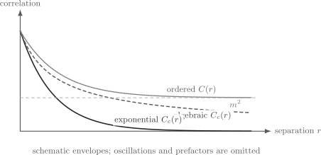
Schematic spatial signatures. A short-range connected correlator can decay exponentially with correlation length $\xi$; a critical correlator can decay algebraically; and a full order-parameter correlator can approach a nonzero plateau $m^2$. Oscillations and algebraic prefactors may accompany any of these envelopes.

Exponential Clustering

In a short-range correlated phase,

$$\left\lvert G^c_{AB}(r) \right\rvert \lesssim C e^{-r/\xi}$$

for large separation, possibly multiplied by a power of $r$. The length $\xi$ sets the scale over which local fluctuations remain appreciably correlated.

For local quantum lattice systems, rigorous exponential-clustering theorems connect a suitable spectral gap and locality assumptions to exponential decay of ground-state connected correlations. The hypotheses matter. Degenerate ground-state sectors, long-range interactions, gapless modes, gauge constraints, and specially chosen nonlocal operators require separate treatment.

Exponential decay does not mean the correlation is exactly zero beyond $\xi$. It means the asymptotic envelope is exponentially suppressed.

Algebraic Correlations

At many continuous critical points and in stable gapless phases,

$$G^c_{OO}(r) \sim \frac{ \cos(\mathbf Q\cdot\mathbf r+\varphi) }{ r^{2\Delta_O} },$$

where $\Delta_O$ is the scaling dimension of the operator in the long-distance theory.

Algebraic decay has no finite exponential correlation length. It does not imply a nonzero long-range plateau because the correlator still tends to zero. It is often called quasi-long-range order in appropriate low-dimensional phases. It signals fluctuations on all scales and often leads to nonanalytic momentum dependence near $\mathbf Q$.

Finite-size data can make a large but finite correlation length resemble a power law over a restricted range. Reliable identification requires multiple sizes, distances well separated from the lattice spacing and boundaries, and comparison of competing functional forms.

Long-Range Order

This overview states the basic criterion. Long-Range Order is the canonical treatment of modulated correlations, volume-averaged definitions, peak scaling, magnetic and crystalline examples, and finite-size caveats.

For a Hermitian order-parameter operator $O_i$, long-range order is indicated by a nonzero asymptotic full correlator,

$$\lim_{\lvert\mathbf r_i-\mathbf r_j\rvert\to\infty} \langle O_i O_j\rangle = m^2 \ne 0,$$

with an appropriate phase factor for modulated order.

In a symmetry-broken pure phase with $\langle O_i\rangle=m$, cluster decomposition gives

$$\langle O_iO_j\rangle \longrightarrow \langle O_i\rangle \langle O_j\rangle,$$

so the connected correlator tends to zero even though the full correlator tends to $m^2$.

In a finite symmetric state, one often has

$$\langle O_i\rangle = 0$$

while

$$\langle O_iO_j\rangle \longrightarrow m^2$$

over distances short compared with the system size. The full two-point function then detects incipient order that the one-point function misses. This is why finite-size studies often use squared order parameters or structure factors rather than inserting symmetry breaking by hand.

For ordering wavevector $\mathbf Q$, define

$$m_{\mathbf Q}^2(L) = \frac{1}{L^2} \sum_{i,j} e^{i\mathbf Q\cdot(\mathbf r_i-\mathbf r_j)} \langle O_iO_j\rangle.$$

If

$$\lim_{L\to\infty} m_{\mathbf Q}^2(L) \gt 0,$$

the scaling is consistent with long-range order. Boundary conditions, aspect ratio, operator normalization, and order of limits must accompany the claim.

Off-diagonal long-range order

Order need not appear in a density-density correlator. For bosons, the one-body density matrix

$$\rho^{(1)}(\mathbf x,\mathbf y) = \left\langle \psi^\dagger(\mathbf x) \psi(\mathbf y) \right\rangle$$

diagnoses one-particle coherence. In an inhomogeneous system, the basis-independent Penrose–Onsager criterion examines whether its largest eigenvalue scales extensively with particle number.

Pair condensation is instead diagnosed through an appropriate two-particle density matrix or pair correlator. The operator and reduced-density-matrix rank must match the type of order being tested. The normalization and contraction rules for $\Gamma^{(2)}$ are fixed in Two-Body Operators.

Clustering and Pure Phases

Cluster decomposition is the asymptotic factorization statement

$$\langle A_XB_Y\rangle - \langle A_X\rangle \langle B_Y\rangle \longrightarrow 0$$

as the separation between bounded regions $X$ and $Y$ grows.

It is a property of the state and operator class, not merely the Hamiltonian. A symmetric mixture of distinct ordered phases can fail to cluster. For instance, an equal mixture of all-up and all-down ferromagnetic sectors has zero one-point magnetization but persistent two-point correlation.

Selecting a pure phase with an infinitesimal field, boundary condition, or thermodynamic-limit prescription can restore clustering within that phase. Thus “subtract the mean and take large distance” can give different-looking answers before and after phase selection even when both descriptions encode the same ordered thermodynamic regime.

Time-Dependent Correlations

For a time-independent Hamiltonian, Heisenberg operators are

$$A_H(t) = e^{iHt/\hbar} A e^{-iHt/\hbar}.$$

An ordinary ordered correlator is

$$C_{AB}(t,t') = \left\langle A_H(t)B_H(t') \right\rangle_\rho.$$

If the state is stationary,

$$[\rho,H] = 0,$$

then simultaneous time translation changes nothing:

$$C_{AB}(t,t') = C_{AB}(t-t',0).$$

This reduction to one time difference does not hold for a generic quench state, driven system, aging state, or explicitly time-dependent Hamiltonian.

Lehmann representation

Let

$$H\lvert n\rangle = E_n\lvert n\rangle, \qquad \rho = \sum_n p_n \lvert n\rangle\langle n\rvert$$

for a stationary state diagonal in energy. Then

$$\begin{aligned} C_{AB}(t) ={}& \sum_{n,m} p_n e^{i(E_n-E_m)t/\hbar} \\ &\times \langle n\lvert A\rvert m\rangle \langle m\lvert B\rvert n\rangle. \end{aligned}$$

The correlator is a weighted sum of transition frequencies. Its Fourier transform,

$$S_{AB}(\omega) = \int_{-\infty}^{\infty} dt\, e^{i\omega t} C_{AB}(t),$$

has the spectral form

$$\begin{aligned} S_{AB}(\omega) ={}& 2\pi \sum_{n,m} p_n \langle n\lvert A\rvert m\rangle \langle m\lvert B\rvert n\rangle \\ &\times \delta\!\left( \omega-\frac{E_m-E_n}{\hbar} \right). \end{aligned}$$

For $B=A^\dagger$, the weights are nonnegative. The locations encode energy differences, while the weights encode matrix elements and state populations.

Temporal decay and recurrence

In a finite isolated system with a discrete spectrum, $C_{AB}(t)$ is generally quasiperiodic rather than irreversibly decaying to zero. Apparent relaxation can arise from dephasing among many frequencies, and recurrences remain possible.

A smooth decay law usually presupposes a thermodynamic or continuum limit, coarse graining, disorder averaging, coupling to an environment, or an observational time window. A conserved component can produce a nondecaying contribution even in a large system.

The phrase “correlation time” is therefore operational. It may describe an exponential envelope, an integral of a normalized correlator, or the width of a spectral feature. The definition must be stated.

The dedicated Time-Dependent Correlations page develops the ordinary two-time function, its Fourier convention, detailed balance, finite-system recurrence, numerical estimation, and nonequilibrium generalization.

Ordering Prescriptions

Several two-point objects use the same operators but answer different questions.

Object	Definition	Main role
ordinary ordered	$\langle A(t)B(0)\rangle$	fluctuations and transition spectra
reversed ordered	$\langle B(0)A(t)\rangle$	complementary transition ordering
symmetrized	$\frac12\langle\{\delta A(t),\delta B(0)\}\rangle$	real noise-like fluctuations
commutator	$\langle[A(t),B(0)]\rangle$	quantum order sensitivity and response kernel
retarded susceptibility	$\frac{i}{\hbar}\theta(t)\langle[A(t),B(0)]\rangle$	causal response to $H'=-fB$
time ordered	$\langle\mathcal T A(t)B(0)\rangle$	perturbation theory and propagators
imaginary time	$\langle\mathcal T_\tau A(\tau)B(0)\rangle_\beta$	thermal equilibrium methods

Green-function conventions often add factors of $-i$, $1/\hbar$, and statistics-dependent signs. The table gives structural roles, not a universal notation standard.

An ordinary correlator is not automatically a response function. Fluctuations and Susceptibilities explains when an integrated equilibrium correlator gives a static thermodynamic response and when Kubo–Mori ordering is required. For a perturbation $H'(t)=-f(t)B$, the retarded susceptibility of $A$ is

$$\chi^R_{AB}(t) = \frac{i}{\hbar} \theta(t) \left\langle [A_H(t),B_H(0)] \right\rangle.$$

Causality enters through $\theta(t)$, and the commutator compares the two operator orders. Retarded and Advanced Response develops the paired support, analyticity, and spectral discontinuity. The Kubo Formula develops the source derivation, sign conventions, and contact-term subtleties.

Momentum and Frequency Space

For a translation-invariant lattice, the static structure factor associated with an operator $O_i$ is commonly

$$S_O(\mathbf q) = \frac{1}{L} \sum_{i,j} e^{-i\mathbf q\cdot(\mathbf r_i-\mathbf r_j)} \langle O_iO_j\rangle.$$

Some authors use the connected correlation instead, subtract elastic or disconnected pieces, or normalize by particle number rather than site number.

A dynamic structure factor can be defined as

$$\begin{aligned} S_O(\mathbf q,\omega) ={}& \frac{1}{2\pi L} \int_{-\infty}^{\infty} dt\, e^{i\omega t} \\ &\times \sum_{i,j} e^{-i\mathbf q\cdot(\mathbf r_i-\mathbf r_j)} \langle O_i(t)O_j(0)\rangle. \end{aligned}$$

The momentum dependence reveals spatial patterns; the frequency dependence resolves transition energies and lifetimes. A sharp dispersing peak can indicate a quasiparticle, while a broad continuum can indicate decay, fractionalization, disorder, or unresolved multi-particle states. Instrumental resolution must be separated from intrinsic width.

Fourier transformation does not remove convention choices. Signs, factors of $2\pi$, volume factors, connected subtraction, and whether $\omega$ is angular frequency or energy all matter.

The dedicated Structure Factors page develops these transforms, elastic and inelastic weight, detailed balance, sum-rule checks, and probe-specific forward models.

Correlations and Conservation Laws

Exact constraints produce sum rules among correlators. If total particle number

$$\hat N = \sum_j n_j$$

is fixed with no fluctuation, then

$$\begin{aligned} \sum_j \langle \delta n_i\delta n_j \rangle &= \left\langle \delta n_i\delta N \right\rangle \\ &= 0. \end{aligned}$$

Positive onsite number variance must be balanced by offsite anticorrelations. Such correlations can arise from a global constraint even without a local interaction.

Likewise, in a total-spin singlet,

$$\mathbf s_{\mathrm{tot}} \lvert\psi\rangle = 0,$$

so

$$\sum_j \left\langle \mathbf s_i\cdot\mathbf s_j \right\rangle = 0.$$

The positive onsite term $s(s+1)$ is balanced by negative correlations with other sites. Sum rules are powerful checks on both analytic derivations and numerical data.

Correlations in Representative Models

Heisenberg model

In the Heisenberg model, spin correlations distinguish ferromagnetic, antiferromagnetic, critical, and gapped regimes. The static structure factor locates dominant ordering wavevectors, while the dynamic structure factor distinguishes sharp magnons from spinon continua.

Hubbard model

In the Hubbard model, useful correlators include:

$$\langle n_i n_j\rangle_c, \qquad \langle\mathbf s_i\cdot\mathbf s_j\rangle, \qquad \langle c_{i\sigma}^\dagger c_{j\sigma}\rangle,$$

as well as pair correlations and time-dependent single-particle Green functions. Green Functions in Many-Body QM explains why the latter connect the $N$-particle state to exact $N\pm1$ sectors. Each correlator diagnoses a different aspect of charge, spin, coherence, or pairing.

t–J model

In the t–J model, the analogous fermion correlators use projected operators. Hole-density, spin, and singlet-pair correlations then probe constrained charge motion and its competition with the spin background. Short-range enhancement on a finite cluster still requires size and boundary scaling before it supports a bulk phase claim.

Kondo model

In the Kondo model, impurity–bath spin correlations diagnose screening, while the conduction-electron $T$-matrix controls impurity scattering. The screening cloud is a spatial correlation profile rather than the wavefunction of one identifiable electron.

Ideal quantum gases

Even without interactions, exchange statistics produces nontrivial field correlations. Wick factorization relates density correlations to one-body coherence in an ideal Gaussian gas. A fixed total particle number also introduces global occupation correlations absent from independent grand-canonical mode sampling.

“Noninteracting” therefore does not mean that every many-particle correlation vanishes.

Correlations, Reduced States, and Information

For two regions $A$ and $B$, every correlator of local operator bases can be computed from the reduced state $\rho_{AB}$. Conversely, a complete operator basis of sufficiently many expectation values reconstructs that reduced state.

In practice, one usually measures only a small subset. Two states can share all one- and selected two-point functions while differing in higher correlations, entanglement, topology, or global constraints.

Correlation functions and information measures answer complementary questions:

• a correlator is operator specific and can retain sign, momentum, and dynamical information;
• mutual information is basis independent and bounds total correlation between regions;
• entanglement measures separate quantum correlation under specified assumptions;
• reduced density matrices contain the complete local information but grow rapidly with subsystem size.

No single scalar measure replaces the full diagnostic set.

Computation and Data Analysis

Exact diagonalization

For eigenstates $\lvert n\rangle$, equal-time correlators are direct expectation values. Time-dependent correlators can use the Lehmann sum or Krylov evolution. Exact spectra provide sharp finite-size delta functions; plotting them with a Lorentzian width introduces a visualization parameter, not a physical lifetime unless a broadening mechanism is modeled.

Tensor-network methods

Matrix-product states efficiently evaluate local and string correlations in many one-dimensional low-entanglement states. Transfer-matrix eigenvalues encode correlation lengths. Real-time or frequency-domain correlators become harder as entanglement grows.

Monte Carlo methods

Imaginary-time and equal-time correlators may be sampled statistically. Error bars are correlated across separation and imaginary time. Analytic continuation to real frequency is ill-conditioned and requires explicit regularization and evidence standards.

Experimental comparison

Before comparing theory and data, include:

• probe form factors and polarization channels;
• finite temperature and ensemble;
• momentum and energy resolution;
• finite observation time;
• trap, boundary, disorder, and domain averaging;
• background subtraction and disconnected elastic contributions;
• the same normalization on both sides.

Agreement in peak position alone does not establish agreement in spectral weight, linewidth, sum rules, or asymptotic scaling.

Practical Workflow

For a correlation-function calculation:

1. Specify the Hamiltonian, state, ensemble, and preparation.
2. Name the operators and all indices.
3. State whether operators are centered.
4. Fix equal time, real time, imaginary time, or contour time.
5. Fix ordinary, symmetrized, time-ordered, normal-ordered, or retarded ordering.
6. State boundary conditions and finite system size.
7. Define Fourier signs and normalization.
8. Check Hermiticity, positivity, symmetry, and conservation-law sum rules.
9. Separate exact delta functions from chosen numerical broadening.
10. Use size, distance, and time scaling before claiming order, a gap, or a lifetime.

Common Mistakes

• Calling $\langle AB\rangle$ connected without subtracting $\langle A\rangle\langle B\rangle$.
• Treating connected and symmetrized correlations as the same object.
• Dropping operator order when $A$ and $B$ do not commute.
• Inferring entanglement from one nonzero connected correlator.
• Concluding that a vanishing one-point order parameter rules out long-range order in a finite symmetric state.
• Using the connected correlator alone to diagnose an ordered symmetric mixture without discussing phase selection.
• Calling algebraic decay long-range order even though the correlator tends to zero.
• Fitting a correlation length over distances comparable with the lattice spacing or system size.
• Assuming a finite isolated system has irreversible temporal decay.
• Interpreting artificial Lorentzian broadening as a measured lifetime.
• Comparing structure factors with different $L$, $N$, or $2\pi$ normalizations.
• Setting continuum coordinates equal without handling contact terms or regularization.
• Treating noninteracting particles as statistically uncorrelated in every ensemble.
• Applying a Gaussian factorization to an interacting non-Gaussian state without testing higher connected functions.
• Ignoring exact sum rules from fixed particle number, total spin, or other conserved quantities.

Exercises

Product-state factorization

Let $\rho=\rho_A\otimes\rho_B$, with $X_A$ acting only on $A$ and $Y_B$ only on $B$. Show that their connected correlation vanishes.

Solution

Using the tensor-product trace,

$$\begin{aligned} \langle X_AY_B\rangle_\rho &= \operatorname{Tr}_{AB} \left[ (\rho_A\otimes\rho_B) (X_A\otimes Y_B) \right] \\ &= \operatorname{Tr}_A(\rho_AX_A) \operatorname{Tr}_B(\rho_BY_B) \\ &= \langle X_A\rangle_\rho \langle Y_B\rangle_\rho. \end{aligned}$$

Therefore

$$\langle X_AY_B\rangle_c = 0.$$

The converse does not follow from one operator pair: vanishing of one selected connected correlator does not prove that the state factorizes.

Classical correlation without entanglement

For

$$\rho_{\mathrm{cl}} = \frac{1}{2} \left( \lvert\uparrow\uparrow\rangle \langle\uparrow\uparrow\rvert + \lvert\downarrow\downarrow\rangle \langle\downarrow\downarrow\rvert \right),$$

compute $\langle s_1^z\rangle$, $\langle s_2^z\rangle$, and $\langle s_1^zs_2^z\rangle_c$. Why does the answer not prove entanglement?

Solution

Each local spin is equally likely to be up or down, so

$$\langle s_1^z\rangle = \langle s_2^z\rangle = 0.$$

Both components have aligned outcomes:

$$\langle s_1^zs_2^z\rangle = \frac{1}{2} \left( \frac{1}{4} + \frac{1}{4} \right) = \frac{1}{4}.$$

Hence

$$\langle s_1^zs_2^z\rangle_c = \frac{1}{4}.$$

The density operator is explicitly a convex mixture of product states, so it is separable. The connected correlation comes from classical uncertainty about which aligned product state was prepared.

Fixed-number sum rule

Suppose $\hat N=\sum_jn_j$ has the exact value $N$ in the state. Prove

$$\sum_j \langle\delta n_i\delta n_j\rangle = 0.$$

What does this imply if $\langle(\delta n_i)^2\rangle\gt0$?

Solution

Exact particle number means

$$\delta N = \hat N-\langle\hat N\rangle$$

annihilates the support of the state. Since

$$\delta N = \sum_j\delta n_j,$$

we have

$$\begin{aligned} \sum_j \langle\delta n_i\delta n_j\rangle &= \left\langle \delta n_i \sum_j\delta n_j \right\rangle \\ &= \langle\delta n_i\delta N\rangle = 0. \end{aligned}$$

The $j=i$ term is the nonnegative onsite variance. If it is positive, the sum of offsite connected correlations must be negative. The global number constraint therefore produces anticorrelation somewhere away from the site.

Lehmann representation

For a stationary state $\rho=\sum_np_n\lvert n\rangle\langle n\rvert$, derive the spectral representation of $\langle A(t)B(0)\rangle$.

Solution

Insert one energy-basis resolution of the identity:

$$\begin{aligned} \langle A(t)B\rangle &= \sum_n p_n \langle n\lvert e^{iHt/\hbar} A e^{-iHt/\hbar} B \rvert n\rangle \\ &= \sum_{n,m} p_n e^{i(E_n-E_m)t/\hbar} A_{nm}B_{mn}. \end{aligned}$$

Fourier transformation uses

$$\int_{-\infty}^{\infty} dt\, e^{ixt} = 2\pi\delta(x)$$

and gives

$$S_{AB}(\omega) = 2\pi \sum_{n,m} p_nA_{nm}B_{mn} \delta\!\left( \omega-\frac{E_m-E_n}{\hbar} \right).$$

Symmetric finite-volume order

Consider the spin state

$$\lvert\mathrm{cat}\rangle = \frac{ \lvert\uparrow\uparrow\cdots\uparrow\rangle + \lvert\downarrow\downarrow\cdots\downarrow\rangle }{\sqrt2}.$$

Compute $\langle s_i^z\rangle$ and $\langle s_i^zs_j^z\rangle$ for distinct sites. What does the result teach about finite-size order diagnostics?

Solution

The two branches contribute opposite local magnetizations, and the cross terms vanish for $L\gt1$. Therefore

$$\langle s_i^z\rangle = 0.$$

In both branches, spins at distinct sites are aligned, so

$$\langle s_i^zs_j^z\rangle = \frac{1}{4}.$$

The one-point function vanishes because the state preserves the spin-flip symmetry, but the two-point function does not decay. Squared order parameters and long-distance correlations can reveal finite-size precursors of symmetry breaking even when a symmetry eigenstate has zero order-parameter expectation.

Structure-factor scaling

Suppose a translation-invariant scalar correlator approaches

$$\langle O_iO_j\rangle \longrightarrow m^2$$

at large separation and define

$$S_O(0) = \frac{1}{L} \sum_{i,j} \langle O_iO_j\rangle.$$

How does $S_O(0)$ scale with $L$?

Solution

There are order $L^2$ distant pairs, and each contributes asymptotically $m^2$. The prefactor is $1/L$, so

$$S_O(0) \sim Lm^2$$

up to subleading short-distance and finite-size corrections. Equivalently,

$$\frac{S_O(0)}{L} \longrightarrow m^2.$$

A peak that grows only as order one under this normalization does not by itself demonstrate long-range order.

Cross-Links

• Correlation Function Definitions — compact convention ledger for equal-time, connected, ordered, response, spectral, and structure-factor objects.
• Many-Body and Quantum Statistical Mechanics
• Core Objects and Notation
• Thermodynamic Limit
• Thermal Density Operators
• Field Operators in Many-Body Models
• Hubbard Model
• Heisenberg Model
• Transverse-Field Ising Model
• XXZ Spin Chain
• Interacting Systems and Approximation Methods
• Interacting Many-Body Systems Overview
• Random Phase Approximation
• Diagrammatic Methods Preview
• Kubo Formula
• Structure Factors
• Green Functions in Many-Body QM
• Thermal Green Functions
• Retarded and Advanced Response
• Susceptibilities
• Spectral Functions
• Fluctuation–Dissipation Theorem
• Sum Rules
• Transport Coefficients Preview
• Expectation Values
• Correlations and Covariance
• Marginals and Correlations
• Many-Body Entanglement Overview
• Wick’s Theorem Preview
• Heisenberg Picture
• Correlation Functions in Path Integrals
• Green Functions and Response Preview
• From Correlation Functions to QFT Observables
• Bath Correlation Functions
• Optical Correlation Functions
• Correlation-Functions Formula Card
• Fourier-Transform Conventions

References

1. O. Penrose and L. Onsager, “Bose–Einstein Condensation and Liquid Helium”, Physical Review 104, 576–584 (1956).
2. R. Kubo, “Statistical-Mechanical Theory of Irreversible Processes. I”, Journal of the Physical Society of Japan 12, 570–586 (1957).
3. C. N. Yang, “Concept of Off-Diagonal Long-Range Order and the Quantum Phases of Liquid He and of Superconductors”, Reviews of Modern Physics 34, 694–704 (1962).
4. M. B. Hastings and T. Koma, “Spectral Gap and Exponential Decay of Correlations”, Communications in Mathematical Physics 265, 781–804 (2006).
5. A. L. Fetter and J. D. Walecka, Quantum Theory of Many-Particle Systems, Dover (2003).
6. G. D. Mahan, Many-Particle Physics, 3rd ed., Springer (2000).
7. A. Altland and B. Simons, Condensed Matter Field Theory, 2nd ed., Cambridge University Press (2010).
8. S. Sachdev, Quantum Phase Transitions, 2nd ed., Cambridge University Press (2011).
9. P. Coleman, Introduction to Many-Body Physics, Cambridge University Press (2015).
10. H. Bruus and K. Flensberg, Many-Body Quantum Theory in Condensed Matter Physics, Oxford University Press (2004).