Interacting Many-Body Systems Overview

An interacting many-body system is a quantum system whose Hamiltonian contains terms that couple two or more microscopic degrees of freedom, so that its dynamics and stationary states generally cannot be reduced to independent one-body problems. A useful schematic form is

H = H_0+V,

where $H_0$ is a chosen solvable or structurally simple part and $V$ contains interactions. This split is not unique. Calling $V$ “small” is meaningful only after specifying a state, an observable, and an energy or length scale against which it is compared.

Interactions are responsible for much of the distinctive structure of quantum matter: screening, bound states, magnetism, superfluidity, superconductivity, collective modes, Mott physics, and quantum criticality. Yet the mere presence of an interaction does not make a problem uniformly hard. Some weak-coupling problems are destabilized by infrared singularities, while some strong-coupling problems possess a controlled expansion in an inverse coupling or a sharply separated low-energy subspace.

The central task is therefore not to attach the label weak or strong to a dimensional constant. It is to identify the relevant dimensionless controls, compare the competing scales, and choose a representation and method adapted to the observable of interest.

Canonical Scope

This page is the canonical overview of interaction regimes in many-body quantum mechanics. It owns:

the physical data needed to specify an interaction;
pairwise continuum and local lattice forms as orientation examples;
short-range, long-range, instantaneous, and effective interactions;
dimensionless definitions of weak, intermediate, and strong coupling;
the distinction between perturbative and nonperturbative behavior;
the emergence of collective degrees of freedom;
a regime-based map of many-body approximation methods.

Neighboring pages retain more focused ownership:

Emergence and Effective Degrees of Freedom owns cross-mechanism variable selection, observable matching, error, and breakdown audits; this page retains interaction regimes, dimensionless controls, collective-behavior orientation, and method selection.
Many-Particle Hamiltonians derives the first- and second-quantized operator grammar.
Two-Body Operators owns pair-counting, matrix-element, reduced-density-matrix, and basis conventions.
Common Many-Body Hamiltonians is the compact formula sheet for standard models.
Lattice Models Overview owns lattice geometry, locality, boundary data, and model families.
Choosing an Approximation Method owns the general few-body decision guide.
Later pages in this chapter own mean field, Hartree, Hartree–Fock, Gross–Pitaevskii, Bogoliubov, BCS, random-phase response, variational state families, large-N saddle methods, many-body perturbation theory, diagrammatic methods, and effective-Hamiltonian derivations.

What Specifies an Interaction?

Writing a potential $v(r)$ or a coupling $U$ is not a complete model specification. At minimum, state:

the microscopic degrees of freedom and their statistics;
the Hilbert space, constraints, and retained bands or modes;
the spatial dimension, geometry, and boundary conditions;
the range, sign, symmetry, and internal-index structure of the interaction;
whether the interaction is instantaneous or frequency dependent;
the ultraviolet regulator or lattice spacing;
density, filling, temperature, and external fields;
the thermodynamic sequence, if a bulk limit is intended;
the observable and scale at which an approximation is claimed;
whether the coupling is microscopic, renormalized, screened, or otherwise effective.

Two Hamiltonians with the same visible coefficient can describe different regimes when their bandwidths, densities, dimensions, or cutoffs differ. Conversely, microscopically different interactions can lead to the same low-energy theory after short-distance details are removed.

Pairwise Continuum Interactions

For $N$ identical particles in a continuum, a common first-quantized Hamiltonian is

H_N = \sum_{i=1}^{N} \left[ \frac{\mathbf p_i^2}{2m} + U_{\mathrm{ext}}(\mathbf r_i) \right] + \sum_{i<j} v(\mathbf r_i-\mathbf r_j).

The restriction $i<j$ counts each unordered pair once. For a translation-invariant, spin-independent interaction, the potential depends only on the relative coordinate. More general interactions can depend on spin, species, orientation, momentum, time, or the center-of-mass position.

In field-operator notation, the same pair structure is

\begin{aligned} V = \frac12 \int d^d x\,d^d y\, &\psi_\alpha^\dagger(\mathbf x) \psi_\beta^\dagger(\mathbf y) v_{\alpha\beta;\gamma\delta} (\mathbf x,\mathbf y) \\ &\times \psi_\delta(\mathbf y) \psi_\gamma(\mathbf x), \end{aligned}

with repeated internal labels summed. The factor $1/2$ again removes pair double counting when the kernel and summation convention are chosen accordingly.

This form does not assume weak coupling. It encodes kinematics and pair structure. Whether it is tractable depends on the potential, statistics, density, dimension, state, and observable.

Pairwise is not the same as independent

A pair interaction is a sum of two-particle operators, but the resulting state need not factor into pairs. One particle can correlate with many others through repeated scattering, and exchange symmetry links amplitudes across all labels.

Even if

V = \sum_{i<j}v_{ij},

the terms $v_{ij}$ and $v_{jk}$ generally share degree of freedom $j$ . The many-body eigenproblem is therefore not a collection of isolated two-body problems.

Two-body interactions can generate higher correlations

Time evolution under a two-body Hamiltonian can generate connected three-point, four-point, and higher correlation functions. A Hamiltonian’s operator rank does not bound the correlation rank of its states.

This is one reason closure schemes matter. Mean-field and Gaussian approximations truncate or factorize a correlation hierarchy; they do not make the exact hierarchy disappear.

Momentum-Space View

For particles in a periodic volume $\Omega$ , define the density mode

\rho_{\mathbf q} = \sum_{\mathbf k,\sigma} c_{\mathbf k+\mathbf q,\sigma}^\dagger c_{\mathbf k,\sigma}.

For a translation-invariant pair potential with Fourier transform $\widetilde v(\mathbf q)$ , the interaction can be written schematically as

V = \frac{1}{2\Omega} \sum_{\mathbf q} \widetilde v(\mathbf q) : \rho_{\mathbf q} \rho_{-\mathbf q} :.

Normal ordering removes the unphysical self-pair contribution in this representation. Equivalently, in a first-quantized density identity one subtracts the $i=j$ term explicitly.

The momentum-space form makes several facts visible:

translation invariance conserves total momentum;
$\widetilde v(\mathbf q)$ weights momentum transfer $\mathbf q$ ;
forward scattering, backscattering, and pairing channels can scale differently;
long-range real-space interactions are singular or sharply structured near small momentum;
screening and collective density response naturally appear in the same variables.

The most useful basis is therefore interaction- and observable-dependent. Real space exposes locality; momentum space exposes conservation laws, Fermi surfaces, and scattering channels.

Local Lattice Interactions

A lattice replaces continuous position by sites, orbitals, or cells. “Local” can mean onsite, finite-range, or rapidly decaying in the chosen lattice basis.

Common examples include:

V_{\mathrm H} = U\sum_i n_{i\uparrow}n_{i\downarrow},

for onsite repulsion between opposite-spin fermions;

V_{\mathrm B} = \frac{U}{2} \sum_i n_i(n_i-1),

for onsite boson repulsion;

V_{\mathrm{dens}} = \sum_{i<j} V_{ij}n_i n_j,

for intersite density interactions; and

V_{\mathrm{spin}} = \sum_{\langle ij\rangle} J_{ij}\, \mathbf S_i\boldsymbol\cdot\mathbf S_j,

for exchange-coupled spins.

These terms compete with one-body hopping, local fields, orbital splittings, and chemical potentials. In the Hubbard model, for example, the ratio of onsite interaction to kinetic bandwidth helps organize the regime, but filling, lattice geometry, temperature, and dimension remain indispensable.

Locality depends on the chosen variables

An onsite interaction in a localized orbital basis becomes a momentum-dependent four-mode scattering term after Fourier transformation. Conversely, a momentum-diagonal quadratic Hamiltonian can be long ranged in real space.

Locality is therefore a statement about both the operator and the representation. Physical locality is usually tied to spatially localized observables, but effective variables can make the same process appear nonlocal.

Constraints can be interactions in disguise

The limit $U\to\infty$ in a lattice model may forbid double occupation. Within the low-energy subspace, the interaction then appears as a kinematic constraint rather than a finite energy term. Virtual excursions outside the constrained subspace can still generate exchange and correlated hopping.

This illustrates a general principle: eliminating high-energy configurations changes both the allowed Hilbert space and the effective operators acting within it.

Short-Range and Long-Range Interactions

Interaction range is not a binary label. Distinguish at least:

contact: idealized support only at coincident points;
finite range: negligible beyond a microscopic distance $R$ ;
short range: sufficiently rapid decay for the intended bulk and infrared arguments;
power law: $v(r)\sim C/r^\alpha$ ;
all to all: every degree of freedom couples with comparable strength;
retarded: the effective interaction depends on time or frequency as well as distance.

For a $d$ -dimensional homogeneous system with

v(r) \sim \frac{C}{r^\alpha},

the large-distance contribution per particle scales like

\int_a^L dr\, r^{d-1-\alpha}.

Consequently:

\begin{array}{c|c} \alpha>d & \text{absolutely summable at large distance},\\ \alpha=d & \text{logarithmic large-distance growth},\\ \alpha<d & \text{power-law large-distance growth}. \end{array}

This counting test is a warning, not a complete thermodynamic theorem. Charge neutrality, screening, alternating signs, boundary shape, background terms, and conditional convergence can change the conclusion. Three-dimensional Coulomb matter is the standard reminder: the bare $1/r$ interaction is not absolutely summable, yet neutral matter can possess a stable thermodynamic limit under appropriate assumptions.

Kac normalization

For an unstructured all-to-all interaction,

V = J\sum_{i<j}O_iO_j,

there are order $N^2$ pairs. A scaling such as

V_{\mathrm{Kac}} = \frac{J}{N} \sum_{i<j}O_iO_j

restores an order- $N$ energy under broad conditions. This makes the energy extensive but does not make the interaction local. Fluctuation structure, dynamics, ensemble equivalence, and finite-size scaling can still differ from short-range systems.

Range changes universality and dynamics

Long-range tails can alter:

whether a thermodynamic limit is shape independent;
the existence and velocity of effective light cones;
collective-mode dispersions;
screening behavior;
critical exponents and upper critical dimensions;
the validity of short-range effective field theories.

The exponent $\alpha$ alone is not enough. Sign, conservation laws, dimensionality, frustration, and the state also matter.

Microscopic, Bare, and Effective Interactions

The interaction used in a calculation is often not a fundamental two-body force.

Bare microscopic interaction

A bare interaction belongs to a specified microscopic model and regulator. Its parameters can depend on the cutoff convention. A bare contact coupling in more than one spatial dimension cannot be interpreted independently of ultraviolet regularization and matching.

Renormalized low-energy interaction

At low collision energy, a complicated short-range potential may be represented by a few scattering parameters. In a dilute three-dimensional gas, the $s$ -wave scattering length $a_s$ controls the leading contact coupling. The canonical scattering definition lives in Scattering Length.

Screened interaction

Other mobile degrees of freedom can rearrange around a perturbation, converting a bare long-range interaction into a scale- and frequency-dependent screened interaction. Screening is collective: it cannot generally be assigned to one isolated pair.

Induced interaction

Eliminating phonons, photons, high-energy orbitals, or another particle species can induce interactions among the retained degrees of freedom. The result can be attractive even if a microscopic Coulomb contribution is repulsive, and it may be retarded rather than instantaneous.

Exchange as an emergent interaction

In a large- $U$ Hubbard regime, hopping through virtual doubly occupied states generates an antiferromagnetic exchange scale

J_{\mathrm{ex}} \sim \frac{4t^2}{U}.

The low-energy spin interaction is not an additional fundamental force. It is produced by statistics, hopping, and virtual high-energy configurations. Effective Hamiltonians in Many-Body Systems owns the projected-sector derivation, generated operators, and validity audit.

Every effective interaction should therefore carry an energy window, retained Hilbert space, and matching prescription.

Coupling Strength Must Be Dimensionless

A dimensional number is never intrinsically small. If a coupling $g$ has units, the numerical statement $g\ll1$ changes when units change.

A meaningful control parameter compares interaction and reference scales:

\lambda = \frac{E_{\mathrm{int}}}{E_{\mathrm{ref}}},

or compares lengths, densities, matrix elements, or response functions in a dimensionless combination.

There is no universal $E_{\mathrm{ref}}$ . It may be a bandwidth, Fermi energy, spectral gap, level spacing, temperature, recoil energy, charging energy, or probe frequency.

System or regime	Useful control	Essential qualification
dilute 3D Bose gas	$n a_s^3$	leading corrections scale as $\sqrt{n a_s^3}$
dilute two-component Fermi gas	$k_{\mathrm F}a_s$	resonance and effective range also matter
single-band Hubbard model	$U/W$ or $U/t$	filling, lattice, and dimension are indispensable
electron gas	$r_s$	definition depends on dimension and density convention
spin model in a field	$J/h$	sign, frustration, anisotropy, and coordination matter
Kondo impurity	$\rho(E_{\mathrm F})J_K$	logarithms grow toward low energy
long-range lattice model	interaction / local scale plus $\alpha$	normalization and thermodynamic sequence matter

The Weakly Interacting Bose Gas Preview is a clean example: weak coupling means $n a_s^3\ll1$ , not merely that a symbol $g$ looks small.

Weak Coupling

A weak-coupling regime is one in which selected observables admit a controlled expansion around a specified reference problem. Schematically,

\mathcal O(\lambda) = \mathcal O_0 + c_1\lambda + c_2\lambda^2 + \cdots.

Control requires more than $|\lambda|\ll1$ :

the coefficients must not grow too rapidly at the relevant order;
small denominators must be absent or treated by degenerate methods;
infrared or ultraviolet logarithms must remain under control;
the observable must be analytic in the chosen expansion parameter over the regime used;
system size and time must not amplify the correction beyond the nominal estimate;
the unperturbed state must represent the correct phase and symmetry sector.

Observable dependence

The same Hamiltonian can be perturbative for one quantity and nonperturbative for another. A weak interaction may produce a small correction to a high-energy spectral moment while reorganizing the ground state at exponentially low energy.

Similarly, short-time dynamics can admit a convergent or asymptotic expansion even when late-time transport requires resummation of repeated collisions.

Degeneracy and dense spectra

The elementary mixing ratio

\eta_{mn} = \frac{|V_{mn}|} {|E_m^{(0)}-E_n^{(0)}|}

must be small for ordinary nondegenerate perturbation theory. In a many-body system, level spacings can shrink rapidly with volume. A matrix element that is microscopically small can therefore mix a dense manifold of states.

This does not make all bulk perturbation theory impossible. It means that one should expand quantities with a well-defined thermodynamic organization, use linked-cluster or Green-function methods, and resum the channels whose denominators become singular.

Large logarithms

An expression of the form

\lambda \ln\!\left( \frac{E_{\mathrm{UV}}}{E_{\mathrm{IR}}} \right)

need not be small even when $|\lambda|\ll1$ . Lowering the infrared scale can invalidate every fixed-order truncation. Renormalization-group flow or channel-specific resummation may then be the controlled description.

Weak Does Not Mean Trivial

Weak attraction near a Fermi surface gives a canonical example. Repeated scattering in the Cooper channel produces a scale-dependent vertex. In a schematic convention,

\Gamma(E) \simeq \frac{g} {1+g\rho_{\mathrm F} \ln(E_c/E)},

where $g<0$ is attractive, $\rho_{\mathrm F}$ is the density of states at the Fermi level, and $E_c$ is a high-energy cutoff. The denominator vanishes at an exponentially small scale,

E_* \sim E_c \exp\!\left[ -\frac{1}{|g|\rho_{\mathrm F}} \right].

No finite power series in $g$ produces this scale. An arbitrarily weak attraction can therefore destabilize the normal Fermi surface at sufficiently low energy under the assumptions of the pairing problem.

This is not a contradiction. The microscopic coupling is weak, while the low-energy logarithm grows until the normal-state expansion must be reorganized around a paired state.

Other weak-coupling reorganizations include:

collective screening from repeated particle–hole processes;
sound from repeated density interactions in a condensate;
the Kondo scale generated by logarithmic flow;
secular growth in nonequilibrium perturbation theory;
bound states whose binding energy is nonanalytic in the coupling.

Intermediate Coupling

An intermediate-coupling regime has no generally useful small ratio in either the interaction or its inverse. It is often the hardest region because several descriptions compete without a controlled hierarchy.

Reliable work in this regime combines constraints rather than relying on one label:

exact symmetries and conservation laws;
variational upper bounds and rigorous inequalities;
sum rules and spectral moments;
high- and low-coupling limiting cases;
finite-size sequences in multiple geometries;
several independent numerical methods where possible;
controlled expansions continued only with explicit uncertainty;
comparison to experimentally accessible correlators and response functions.

“Strongly correlated” is often used for such systems, but it has no universal numerical threshold. A trustworthy statement specifies which independent-particle, mean-field, or quasiparticle description fails and which observable demonstrates that failure.

Strong Coupling

Strong coupling means that an interaction scale dominates a chosen competing scale. It does not mean that every quantity is uncontrolled.

Suppose

H = H_U+T, \qquad U\gg t,

where $H_U$ separates low- and high-energy local configurations by energy of order $U$ , while $T$ mixes them with matrix elements of order $t$ .

The low-energy theory can admit an expansion in

\frac{t}{U} \ll 1.

To second order, virtual high-energy excursions generate terms of order $t^2/U$ . At half filling in the repulsive single-band Hubbard model, this yields antiferromagnetic superexchange with $J_{\mathrm{ex}}=4t^2/U$ under the standard nearest-neighbor convention.

The original model is strongly coupled relative to hopping, yet its low-energy Hamiltonian is perturbatively controlled in the inverse coupling. The correct unperturbed problem is the local interacting manifold, not the free-particle band.

Strong-coupling caveats

A projected Hamiltonian describes only energies well below the eliminated gap.
Degeneracy inside the low-energy manifold requires degenerate perturbation theory.
Effective observables must be transformed along with the Hamiltonian.
The expansion can fail when the gap closes or doping introduces new low-energy configurations.
A large bare coupling need not imply a simple low-energy state; frustration and competing exchanges may remain.

Perturbative and Nonperturbative Regimes

These terms describe analytic structure, not merely magnitude.

Perturbative contribution

A perturbative contribution is represented by a controlled series in a declared parameter, often around $\lambda=0$ or $1/\lambda=0$ :

\mathcal O \sim \sum_{n=0}^{\infty} c_n\lambda^n.

The series may converge or may be asymptotic. An asymptotic series can still be highly predictive when optimally truncated and accompanied by an error estimate.

Nonperturbative contribution

A contribution such as

\exp\!\left(-\frac{A}{\lambda}\right)

has a vanishing Taylor series at $\lambda=0$ and is invisible at every finite perturbative order. Nonperturbative structure can also arise from:

a change of phase or symmetry sector;
tunneling between semiclassical configurations;
topological sectors;
bound-state formation;
infrared flow to a new fixed point;
constraints that reorganize the Hilbert space;
level crossings or thermodynamic-limit nonanalyticities.

The labels are not synonyms

The following implications are false in general:

\begin{gathered} \text{weak coupling} \not\Rightarrow \text{all observables perturbative}, \\ \text{strong coupling} \not\Rightarrow \text{no controlled expansion}, \\ \text{nonperturbative} \not\Rightarrow \text{numerically large}. \end{gathered}

An exponentially small gap is nonperturbative but small. A leading strong-coupling exchange can be perturbative in $t/U$ and physically decisive.

Crossovers, Instabilities, and Phases

A coupling ratio can mark several different phenomena.

Crossover

A crossover is a smooth change in the most useful description. No thermodynamic-limit nonanalyticity is required. A gas can cross from classical to degenerate statistics, or a quasiparticle can evolve from long lived to overdamped.

Instability of a reference state

A susceptibility divergence or negative mode can show that the chosen reference state is unstable. This indicates the need for a reorganized state or effective theory, but it does not by itself determine the final phase.

Phase transition

A sharp phase transition is a bulk statement involving nonanalytic thermodynamic-limit behavior, a change of symmetry realization, topological structure, or another phase diagnostic. Quantum Phase Transitions owns the zero-temperature definition and finite-size cautions.

One should not infer a phase transition merely because a perturbative approximation fails. The method may fail before, at, or after the physical transition, and it can fail even in a single smooth phase.

Competing Preferred Bases

Many-body difficulty often comes from noncommuting terms that prefer incompatible states.

For a lattice Hamiltonian

H = H_{\mathrm{kin}}+H_{\mathrm{int}},

the kinetic term may be diagonal in momentum occupation, while the interaction is simplest in localized occupation. If

[H_{\mathrm{kin}},H_{\mathrm{int}}] \ne 0,

no basis simultaneously minimizes or diagonalizes both parts.

The transverse-field Ising model presents the same structure in spin language: exchange favors $z$ -ordered configurations, while the transverse field favors $x$ polarization. The competition, not merely the size of either matrix, produces quantum fluctuations and possible criticality.

This observation guides approximations. Start from the term that defines a controlled manifold, but test whether the neglected term mixes nearby states strongly.

Correlations as the Signature of Interaction

For observables $A$ and $B$ , define the connected correlation

C_{AB} = \langle AB\rangle - \langle A\rangle \langle B\rangle.

Interactions often generate nonzero connected correlations, but several qualifications matter:

exchange statistics produces correlations even in noninteracting gases;
constraints can correlate occupations without an explicit finite interaction term;
a product mean-field state sets selected connected correlations to zero by construction;
a vanishing two-point connected correlator does not imply absence of higher correlations;
correlation is not automatically entanglement.

Correlation Functions Overview owns the hierarchy, orderings, Fourier conventions, and relation to measured response.

Coupling derivatives as diagnostics

For

H(g) = H_0+gV,

the Hellmann–Feynman relation for a nondegenerate normalized eigenstate gives

\frac{dE_n}{dg} = \langle n(g)|V|n(g)\rangle.

At finite temperature, with

F(g) = -\frac{1}{\beta} \ln\operatorname{Tr} e^{-\beta H(g)},

one similarly has

\frac{\partial F}{\partial g} = \langle V\rangle_{\beta,g}.

These identities connect energy or free-energy changes directly to interaction observables. They are useful checks for analytic approximations, finite-difference calculations, and numerical simulations.

Emergence of Collective Behavior

Interactions couple microscopic motion so that the long-wavelength degrees of freedom need not resemble the original particles.

Screening

An external charge perturbs many particles, whose induced density modifies the field seen by later particles. The resulting screened interaction depends on collective response and often on both momentum and frequency.

Collective modes

Poles or sharp peaks in response functions can represent coherent oscillations of density, phase, spin, or an order parameter. Their dispersion and linewidth, rather than a microscopic trajectory, define the excitation. Collective Modes develops the shared coordinate, polarization, response-matrix, propagation, and damping framework.

Quasiparticles

Interactions dress a microscopic particle with surrounding polarization and virtual excitations. A quasiparticle is useful when a spectral peak remains narrow compared with its excitation energy. Strong interaction does not automatically destroy quasiparticles, and weak interaction does not guarantee them at every energy. Quasiparticles Overview gives the full taxonomy, effective-particle data, wave-packet criteria, and breakdown tests.

Bound states and pairing

Repeated attraction can produce molecular, excitonic, Cooper-pair, or other composite degrees of freedom. The bound object may be the natural low-energy variable even though the Hamiltonian was written in terms of its constituents.

Order and rigidity

Interactions can correlate many degrees of freedom into an ordered state with stiffness against twists or deformations. Magnetization, condensate phase, density modulation, and pairing amplitude are examples, but not every phase is characterized by a local order parameter.

Effective interactions among emergent objects

The story repeats at a new scale. Phonons scatter, quasiparticles interact, domain walls bind, and collective modes decay. Emergence does not mean that interactions vanish; it means that the useful degrees of freedom and couplings have changed.

Scale Dependence

An interaction can appear weak at one scale and strong at another. A coarse-grained description integrates out high-energy modes and changes the effective couplings among the retained modes.

The qualitative flow can be:

toward zero, making the interaction irrelevant at long distance;
toward a finite fixed point, producing universal interacting behavior;
toward strong coupling, signaling a new scale, instability, or change of variables;
along a line of fixed points, giving continuously varying exponents or parameters.

Renormalization Group Preview develops this scale-dependent language into coarse-graining maps, beta functions, and fixed-point stability. Even before a full calculation, it forces three questions:

At what resolution is the coupling defined?
Which modes have already been eliminated?
Which observables remain sensitive to the microscopic value?

Regime and Method Map

No single axis selects a many-body method. Interaction range, statistics, density, dimension, symmetry, temperature, and the target observable all enter.

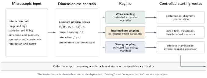
Flow from microscopic interaction data through dimensionless controls and coupling regimes to controlled many-body methods and collective outputs. — Microscopic couplings acquire meaning only through dimensionless ratios and scale hierarchies. Weak, intermediate, and strong coupling each admit several routes; the arrows are starting points rather than universal prescriptions. Collective behavior feeds back into the useful low-energy variables.

The map deliberately sends more than one arrow from each regime. Mean field can be useful at weak coupling, large coordination, large occupancy, or large- $N$ even when the microscopic coupling is not tiny. Numerical methods are not reserved for “strong coupling,” and perturbation theory can be organized around an interacting strong-coupling limit.

Structure-Matched Starting Methods

Structure of the problem	Natural starting route	Main validation question
weak coupling, no singular channels	many-body perturbation theory	are corrections and residuals small?
weak coupling with large logarithms	resummation or renormalization group	which channel flows first?
condensate with small depletion	Gross–Pitaevskii plus Bogoliubov fluctuations	is depletion parametrically small?
product-like order or large coordination	self-consistent mean field	are connected fluctuations controlled?
fermionic Slater-determinant regime	Hartree–Fock	are correlation energies and instabilities small?
dominant local interaction with a gap	projection and strong-coupling expansion	is the eliminated sector well separated?
controlled large parameter	large-N and saddle-point methods or semiclassics	are finite-parameter corrections bounded?
one-dimensional low-entanglement ground state	matrix-product-state methods	are bond dimension and finite size converged?
nonnegative statistical weights	quantum Monte Carlo	are finite-size and continuation errors controlled?
small symmetry-resolved Hilbert space	exact diagonalization or Krylov methods	do observables scale consistently with size?
no evident small parameter	cross-method benchmarking	which independent constraints agree?

The method should be selected after naming the observable. Ground-state energy, order parameter, high-frequency moment, low-frequency conductivity, long-time relaxation, and entanglement growth can demand different approximations for the same Hamiltonian.

A Practical Regime Checklist

Before calculating, answer the following.

Define the model

What is the retained Hilbert space?
Which particle statistics and constraints apply?
Is the interaction bare, matched, screened, or induced?
Which cutoff, lattice spacing, or bandwidth accompanies it?

Identify scales

What are the kinetic, interaction, gap, thermal, and probe scales?
Which dimensionless ratios compare them?
Does the answer change with density, filling, or system size?
Are there large logarithms or small denominators?

Identify structure

Which symmetries block-diagonalize the problem?
Is there a separated low-energy manifold?
Is the state expected to be product-like, Gaussian, quasiparticle-like, or highly entangled?
Are interactions short ranged, screened, frustrated, or retarded?

Validate the output

Does the result reproduce noninteracting and solvable limits?
Are conservation laws, Ward identities, and sum rules respected?
Are observables insensitive to the regulator after matching?
Do finite-size, basis, and truncation sequences converge?
Does a second method agree in an overlap regime?
Is the claimed uncertainty smaller than the physical effect?

Common Mistakes

Calling a dimensional coupling “small” without forming a dimensionless ratio.
Treating $H=H_0+V$ as a unique physical decomposition.
Assuming pairwise interactions produce only pair correlations.
Confusing short range with weak coupling.
Confusing long range with strong coupling.
Ignoring density, filling, dimension, or bandwidth when quoting $U/t$ or another ratio.
Using a contact interaction without a regulator and matching prescription.
Replacing a bare Coulomb interaction by a screened static potential at frequencies where retardation matters.
Applying nondegenerate perturbation theory to a dense or degenerate manifold.
Assuming weak coupling excludes exponentially small nonperturbative scales.
Assuming strong coupling excludes a controlled inverse-coupling expansion.
Calling the failure of an approximation a phase transition.
Treating a finite-size avoided crossing as a bulk singularity.
Projecting out high-energy states without transforming observables.
Trusting mean-field self-consistency as an error estimate.
Inferring absence of interaction effects from a small energy correction alone.
Calling every interaction-generated correlation entanglement.
Applying an effective interaction outside its energy window.
Quoting a phase diagram without the thermodynamic sequence and boundary data.

Exercises

Pair counting and extensivity

Consider

V_N = J_N \sum_{i<j}O_iO_j,

where typical pair expectations remain order one. Determine the scaling of $J_N$ required for an extensive interaction energy in an unstructured all-to-all model.

Solution

There are

\frac{N(N-1)}{2}

unordered pairs. With $J_N$ independent of $N$ , a typical interaction expectation therefore scales as $N^2$ .

Choose

J_N = \frac{J}{N}

to obtain

\langle V_N\rangle \sim \frac{J}{N}N^2 \sim JN.

This Kac-type normalization makes the energy extensive. It does not make the model local or guarantee ordinary short-range thermodynamics.

Density representation of a pair interaction

For first-quantized density modes

\rho_{\mathbf q} = \sum_{j=1}^{N} e^{-i\mathbf q\boldsymbol\cdot\mathbf r_j},

show that $\rho_{\mathbf q}\rho_{-\mathbf q}$ contains both pair terms and a self term.

Solution

Multiplication gives

\begin{aligned} \rho_{\mathbf q} \rho_{-\mathbf q} &= \sum_{i,j} e^{-i\mathbf q\boldsymbol\cdot\mathbf r_i} e^{i\mathbf q\boldsymbol\cdot\mathbf r_j} \\ &= N + \sum_{i\ne j} e^{-i\mathbf q\boldsymbol\cdot (\mathbf r_i-\mathbf r_j)}. \end{aligned}

The $i=j$ terms each equal one and sum to $N$ . The remaining ordered-pair sum counts each unordered pair twice after combining $\mathbf q$ and $-\mathbf q$ . Normal ordering or explicit subtraction removes the self term in the interaction Hamiltonian.

Power-law summability

For $v(r)\sim C/r^\alpha$ in $d$ dimensions, evaluate the large- $L$ behavior of

I(L) = \int_a^L dr\, r^{d-1-\alpha}.

Solution

For $\alpha\ne d$ ,

I(L) = \frac{ L^{d-\alpha} - a^{d-\alpha} }{d-\alpha}.

Thus $I(L)$ converges as $L\to\infty$ when $\alpha>d$ and grows as $L^{d-\alpha}$ when $\alpha<d$ . At $\alpha=d$ ,

I(L) = \ln\!\left(\frac{L}{a}\right).

This establishes the absolute-summability test. Neutrality, oscillating signs, screening, and boundary prescriptions can still modify the thermodynamic conclusion.

Why a dimensional coupling is not weak by itself

In three dimensions, a contact interaction for nonrelativistic bosons is often written with

g = \frac{4\pi\hbar^2 a_s}{m}.

Explain why $g\ll1$ is meaningless and construct the dilute-gas parameter from $n$ and $a_s$ .

Solution

The coupling $g$ has units of energy times volume, so its numerical value changes under a change of units. The density $n$ has units of inverse volume, while $a_s$ has units of length. The dimensionless combination is

\gamma = n a_s^3.

The dilute weak-correlation regime is $\gamma\ll1$ . Equivalently, the scattering length is much smaller than the mean spacing $n^{-1/3}$ . The leading beyond-mean-field expansion is organized in powers involving $\sqrt\gamma$ , not in the bare numerical value of $g$ .

A weak-coupling nonperturbative scale

Let

E_*(\lambda) = E_c e^{-1/\lambda}, \qquad \lambda>0.

Show that every derivative of $E_*$ at $\lambda=0^+$ vanishes, even though $E_*>0$ for every $\lambda>0$ .

Solution

Each derivative has the form

\frac{d^n E_*}{d\lambda^n} = E_c e^{-1/\lambda} P_n\!\left(\frac{1}{\lambda}\right),

where $P_n$ is a polynomial. The exponential decays faster than any inverse power grows, so

\lim_{\lambda\to0^+} \frac{d^n E_*}{d\lambda^n} = 0

for every finite $n$ . The Taylor series about zero is therefore identically zero and cannot reproduce $E_*$ at positive coupling. The scale is nonperturbative in $\lambda$ even though it is exponentially small.

Strong-coupling superexchange scale

In a half-filled two-site repulsive Hubbard model with $U\gg t$ , hopping connects singly occupied states to intermediate doubly occupied states. Use second-order dimensional reasoning to obtain the scale and sign of the singlet–triplet splitting.

Solution

A virtual hop has amplitude $t$ and reaches a state whose energy is higher by $U$ . Returning to the low-energy sector gives a second-order scale

\frac{t^2}{U}.

The spin singlet can use both virtual double-occupation channels, while Pauli exclusion blocks the corresponding processes for the triplet in the single-orbital model. The singlet is therefore lowered relative to the triplet.

Matching to

H_{\mathrm{eff}} = J_{\mathrm{ex}} \left( \mathbf S_1\boldsymbol\cdot\mathbf S_2 - \frac14 \right)

gives

J_{\mathrm{ex}} = \frac{4t^2}{U}>0.

The positive sign is antiferromagnetic in this convention. The expansion is controlled by $t/U$ , despite the original model being in a strong- $U$ regime.

Mean-field factorization and the discarded term

Let $A=\langle A\rangle+\delta A$ and $B=\langle B\rangle+\delta B$ . Derive the exact decomposition of $AB$ and identify the mean-field approximation.

Solution

Expanding gives

\begin{aligned} AB = {}& \langle A\rangle B + A\langle B\rangle - \langle A\rangle \langle B\rangle \\ &+ \delta A\,\delta B. \end{aligned}

The simplest mean-field decoupling drops the quadratic fluctuation operator:

AB \longrightarrow \langle A\rangle B + A\langle B\rangle - \langle A\rangle \langle B\rangle.

Self-consistency determines the expectations in the resulting one-body problem. The omitted $\delta A\,\delta B$ term is precisely where connected fluctuations enter; self-consistency alone does not prove that it is small.

Failure of a naive small-coupling test

Two unperturbed states have spacing $\Delta$ and are coupled by a matrix element $v$ . The Hamiltonian in that subspace is

H = \begin{pmatrix} 0 & v\\ v^* & \Delta \end{pmatrix}.

Find the dimensionless mixing parameter and state when nondegenerate perturbation theory fails.

Solution

The eigenvalues are

E_\pm = \frac{\Delta}{2} \pm \sqrt{ \frac{\Delta^2}{4} + |v|^2 }.

The relevant ratio is

\eta = \frac{|v|}{|\Delta|}.

For $\eta\ll1$ , ordinary nondegenerate corrections are controlled. When $\eta$ is order one or larger, the states mix strongly and the two-dimensional block should be diagonalized exactly. A small dimensional value of $v$ is irrelevant if the spacing is even smaller.

Key Takeaways

An interaction regime is defined by dimensionless ratios, scales, states, and observables, not by a coupling symbol alone.
Pairwise Hamiltonians can generate correlations of all orders.
Short range, weak coupling, locality, and perturbative control are distinct properties.
Weak interactions can create nonperturbative low-energy scales through degeneracy and infrared enhancement.
Strong coupling can possess a controlled inverse-coupling expansion and a simpler effective Hilbert space.
Intermediate coupling usually requires independent constraints and cross-method benchmarking.
Effective interactions must be accompanied by their cutoff, matching, retained variables, and energy window.
Collective behavior changes the useful degrees of freedom; screening, order, bound states, and quasiparticles are many-body outcomes rather than extra microscopic inputs.
Method selection is observable- and scale-dependent.

Cross-Links

References

P. W. Anderson, “More Is Different,” Science 177, 393–396 (1972), doi:10.1126/science.177.4047.393.
J. Hubbard, “Electron Correlations in Narrow Energy Bands,” Proceedings of the Royal Society A 276, 238–257 (1963), doi:10.1098/rspa.1963.0204.
J. Bardeen, L. N. Cooper, and J. R. Schrieffer, “Theory of Superconductivity,” Physical Review 108, 1175–1204 (1957), doi:10.1103/PhysRev.108.1175.
K. G. Wilson, “The Renormalization Group: Critical Phenomena and the Kondo Problem,” Reviews of Modern Physics 47, 773–840 (1975), doi:10.1103/RevModPhys.47.773.
E. H. Lieb and J. L. Lebowitz, “The Constitution of Matter: Existence of Thermodynamics for Systems Composed of Electrons and Nuclei,” Advances in Mathematics 9, 316–398 (1972), doi:10.1016/0001-8708(72)90023-0.
A. L. Fetter and J. D. Walecka, Quantum Theory of Many-Particle Systems, Dover (2003).
G. D. Mahan, Many-Particle Physics, 3rd ed., Springer (2000), doi:10.1007/978-1-4757-5714-9.
P. Coleman, Introduction to Many-Body Physics, Cambridge University Press (2015), doi:10.1017/CBO9781139020916.
A. Altland and B. D. Simons, Condensed Matter Field Theory, 2nd ed., Cambridge University Press (2010), doi:10.1017/CBO9780511789984.
A. Auerbach, Interacting Electrons and Quantum Magnetism, Springer (1994), doi:10.1007/978-1-4612-0869-3.
P. Nozières and D. Pines, The Theory of Quantum Liquids, Volume I: Normal Fermi Liquids, Westview Press (1999).
A. C. Hewson, The Kondo Problem to Heavy Fermions, Cambridge University Press (1993), doi:10.1017/CBO9780511470752.