BCS Mean-Field Theory

BCS mean-field theory is the self-consistent quadratic approximation to a fermionic pairing Hamiltonian. It replaces pair scattering among many momentum states by a complex pair field, diagonalizes the resulting particle–hole Hamiltonian with a fermionic Bogoliubov transformation, and determines that field from the state of the quasiparticles it creates.

The logical chain is

$$\text{Fermi surface} \longrightarrow \text{Cooper instability} \longrightarrow \text{pairing saddle} \longrightarrow \text{gapped quasiparticles}.$$

Each arrow carries an assumption. A Fermi surface supplies a large phase space of nearly degenerate pair states. An attractive eigenvalue in a pairing channel produces a logarithmic normal-state instability. Mean-field factorization selects a saddle in that channel. The quadratic saddle then supports Bogoliubov quasiparticles. None of these steps proves that every interacting fermion system is a weak-coupling BCS state.

The exact reduced pairing Hamiltonian conserves particle number. Its familiar mean-field representative does not: it mixes sectors differing by two particles while preserving fermion parity. This distinction is essential in finite systems and whenever the phrase “broken U(1)” is used.

Canonical Scope

This page is the canonical home for:

• the reduced pairing Hamiltonian as the microscopic starting point for anomalous mean-field decoupling;
• the Cooper problem as a preview of the pairing instability;
• anomalous mean-field decoupling and its subtraction constant;
• the BCS variational state;
• the fermionic Nambu Hamiltonian and Bogoliubov quasiparticles;
• coherence factors and anomalous averages;
• the finite-temperature gap equation;
• the number equation at fixed density;
• weak-coupling formulas for the zero-temperature gap and transition temperature;
• the grand potential and condensation energy;
• the relation between the symmetry-breaking saddle and exact number conservation;
• the assumptions, checks, and failure modes of BCS mean field.

Reduced BCS Model owns the exact finite-level Hamiltonian, seniority sectors, Richardson equations, and fixed-number benchmark. BCS Model is the compact model card. Bogoliubov Theory owns the general algebraic contrast between bosonic paraunitary and fermionic unitary transformations. Hubbard–Stratonovich Transformation Preview owns the exact complex Gaussian identity that can introduce a pairing field before the BCS saddle is selected. Number Operators and Conserved Quantities owns the detailed number-charge bookkeeping. Ginzburg–Landau Theory owns the spatial material phenomenology obtained near $T_c$; other detailed materials, vortices, and unconventional pairing also belong in Quantum Matter.

For a material claim, Superfluidity and Superconductivity selects among phase, response, defect, weak-link, proximity, and topology routes; this page remains the canonical pairing-saddle derivation.

Conventions

We use the grand Hamiltonian

$$K = H-\mu\widehat N,$$

and define

$$\xi_{\mathbf k} = \epsilon_{\mathbf k}-\mu.$$

The elementary model assumes:

• two fermionic internal states denoted $\uparrow$ and $\downarrow$;
• time-reversal- and inversion-symmetric dispersion, so $\xi_{-\mathbf k}=\xi_{\mathbf k}$;
• zero-center-of-mass pairing of $\mathbf k\uparrow$ with $-\mathbf k\downarrow$;
• an even form factor $w_{\mathbf k}=w_{-\mathbf k}$;
• an attractive coupling $g>0$ in the sign convention used below;
• system volume $\mathcal V$;
• a single-spin density of states per unit volume, denoted $\nu(\xi)$.

For the elementary isotropic model,

$$w_{\mathbf k} = \begin{cases} 1, & |\xi_{\mathbf k}|<\omega_{\mathrm c}, \\ 0, & |\xi_{\mathbf k}|>\omega_{\mathrm c}. \end{cases}$$

Here $\omega_{\mathrm c}$ is an interaction cutoff, not automatically a universal physical constant. In the simplest phonon-window model it is of order a characteristic phonon energy. In a continuum contact model, a bare cutoff and coupling must instead be eliminated in favor of a physical scattering parameter.

Momentum sums run over one label $\mathbf k$ for each ordered pair of spin orbitals $(\mathbf k\uparrow,-\mathbf k\downarrow)$. With this convention, every spin orbital appears once across the product state and quasiparticle sum.

From an Interaction to the Reduced Pairing Model

A general two-body interaction contains many scattering channels. The reduced BCS model retains scattering of time-reversed pairs with zero total momentum. Define

$$b_{\mathbf k}^\dagger = c_{\mathbf k\uparrow}^\dagger c_{-\mathbf k\downarrow}^\dagger, \qquad b_{\mathbf k} = c_{-\mathbf k\downarrow} c_{\mathbf k\uparrow}.$$

The collective pair operator is

$$B^\dagger = \sum_{\mathbf k} w_{\mathbf k}b_{\mathbf k}^\dagger.$$

The reduced grand Hamiltonian is

$$\begin{aligned} K_{\mathrm{red}} ={}& \sum_{\mathbf k,\sigma} \xi_{\mathbf k} c_{\mathbf k\sigma}^\dagger c_{\mathbf k\sigma} \\ &- \frac{g}{\mathcal V} B^\dagger B. \end{aligned}$$

Equivalently,

$$\begin{aligned} K_{\mathrm{red}} ={}& \sum_{\mathbf k,\sigma} \xi_{\mathbf k} c_{\mathbf k\sigma}^\dagger c_{\mathbf k\sigma} \\ &- \frac{g}{\mathcal V} \sum_{\mathbf k,\mathbf k'} w_{\mathbf k}w_{\mathbf k'} b_{\mathbf k}^\dagger b_{\mathbf k'}. \end{aligned}$$

The factor $1/\mathcal V$ makes the interaction energy extensive when $g$ is held fixed in the thermodynamic limit.

What has been discarded

The reduction is physical input, not an operator identity. It suppresses or absorbs:

• density and exchange terms;
• finite-center-of-mass pairing;
• retardation of the interaction;
• detailed frequency and momentum dependence;
• Coulomb pseudopotential effects;
• competing spin, charge, and magnetic channels;
• self-energy corrections to the normal-state dispersion.

In a conventional weak-coupling application, some of those effects motivate the attractive low-energy interaction and renormalize $\xi_{\mathbf k}$ and $g$. They are not derived by solving the reduced Hamiltonian.

Exact Number Symmetry

The pair operators carry number charges

$$[ \widehat N, b_{\mathbf k}^\dagger ] = 2b_{\mathbf k}^\dagger, \qquad [ \widehat N, b_{\mathbf k} ] = -2b_{\mathbf k}.$$

The pair-scattering product is neutral:

$$[ \widehat N, b_{\mathbf k}^\dagger b_{\mathbf k'} ] = 0.$$

Therefore

$$[ \widehat N, K_{\mathrm{red}} ] = 0.$$

The exact model moves a pair from one time-reversed orbital pair to another. It does not create particles from nothing. The exact Hilbert space decomposes into fixed-$N$ sectors, and the reduced Hamiltonian preserves each one.

The Hamiltonian also preserves fermion parity,

$$P_F = (-1)^{\widehat N}.$$

Parity will remain a symmetry even after the usual mean-field approximation mixes sectors differing by two particles.

Pair Operators Are Not Elementary Bosons

For one momentum label,

$$[ b_{\mathbf k}, b_{\mathbf k}^\dagger ] = 1 - n_{\mathbf k\uparrow} - n_{-\mathbf k\downarrow}.$$

The right-hand side is state dependent. Moreover,

$$\left( b_{\mathbf k}^\dagger \right)^2 = 0.$$

One pair orbital can be empty, paired, or blocked by a singly occupied fermionic mode. Pair operators for distinct labels commute because they have even fermion parity, but each label retains a hard-core constraint.

This is why a weak-coupling Cooper pair should not be pictured as a pointlike elementary boson. Its constituents occupy a broad, Pauli-constrained superposition of momentum states.

Pseudospin representation

Define Anderson pseudospins

$$S_{\mathbf k}^+ = b_{\mathbf k}^\dagger, \qquad S_{\mathbf k}^- = b_{\mathbf k},$$

and

$$S_{\mathbf k}^z = \frac{1}{2} \left( n_{\mathbf k\uparrow} + n_{-\mathbf k\downarrow} - 1 \right).$$

On the empty and paired subspace, these obey a spin-$1/2$ algebra. Apart from a constant and blocked levels,

$$K_{\mathrm{red}} = 2\sum_{\mathbf k} \xi_{\mathbf k}S_{\mathbf k}^z - \frac{g}{\mathcal V} \sum_{\mathbf k,\mathbf k'} w_{\mathbf k}w_{\mathbf k'} S_{\mathbf k}^+S_{\mathbf k'}^-.$$

This representation exposes the competition between energy, which favors pseudospins pointing according to the sign of $\xi_{\mathbf k}$, and pairing, which favors transverse alignment. It also connects the reduced model to the exact Richardson solution. Mean field is not the only possible treatment of the reduced Hamiltonian.

Cooper Instability Preview

The Cooper problem asks what happens when two additional fermions interact attractively above an inert filled Fermi sea. Use the trial state

$$|\Psi\rangle = \sum_{\mathbf k}^{0<\xi_{\mathbf k}<\omega_{\mathrm c}} \phi_{\mathbf k} b_{\mathbf k}^\dagger |\mathrm{FS}\rangle.$$

Let the pair energy relative to $2\mu$ be $-E_{\mathrm b}$, with $E_{\mathrm b}>0$. For a constant attraction in the shell, the Schrödinger equation gives

$$\left( 2\xi_{\mathbf k} + E_{\mathrm b} \right) \phi_{\mathbf k} = \frac{g}{\mathcal V} \sum_{\mathbf k'} \phi_{\mathbf k'}.$$

Hence

$$\phi_{\mathbf k} \propto \frac{1}{ 2\xi_{\mathbf k}+E_{\mathrm b} }.$$

The consistency condition is

$$1 = \frac{g}{\mathcal V} \sum_{\mathbf k}^{0<\xi_{\mathbf k}<\omega_{\mathrm c}} \frac{1}{ 2\xi_{\mathbf k}+E_{\mathrm b} }.$$

For an approximately constant single-spin density of states $\nu(0)$,

$$1 = \frac{g\nu(0)}{2} \ln \left( \frac{ 2\omega_{\mathrm c}+E_{\mathrm b} }{ E_{\mathrm b} } \right).$$

Solving gives

$$E_{\mathrm b} = \frac{ 2\omega_{\mathrm c} }{ \exp[ 2/(g\nu(0)) ] - 1 }.$$

At weak coupling,

$$E_{\mathrm b} \simeq 2\omega_{\mathrm c} \exp \left[ - \frac{2}{g\nu(0)} \right].$$

The logarithm diverges as $E_{\mathrm b}\to0^+$. In the idealized continuum problem, every $g>0$ therefore produces a bound pair above the Fermi sea.

What the Cooper problem establishes

It establishes that the normal Fermi sea is singularly susceptible to attraction in the pair channel. A large set of pair states close to the Fermi surface are nearly degenerate, so repeated scattering cannot be represented by a regular finite-order expansion in $g$. Perturbation Theory in Many-Body Systems places this logarithm in the broader map of infrared failures and resummations.

What it does not establish

The Cooper problem:

• freezes the Fermi sea;
• treats only one added pair;
• uses only unoccupied states above the surface;
• does not determine a many-body order parameter;
• does not produce the BCS number equation or thermodynamics.

The exponent differs from the BCS gap exponent because the many-body gap equation uses coherent particle and hole states on both sides of the Fermi surface.

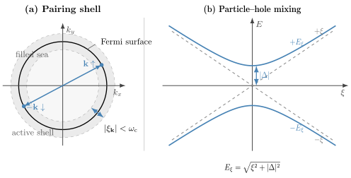
Left: the reduced model couples time-reversed states within an energy shell around the Fermi surface. Right: the normal particle and hole branches $\pm\xi$ cross at the Fermi surface, while a nonzero pair field produces $E=\sqrt{\xi^2+|\Delta|^2}$ and an excitation gap $|\Delta|$.

Anomalous Mean-Field Decoupling

Write

$$B = \langle B\rangle + \delta B.$$

Then

$$\begin{aligned} B^\dagger B ={}& \langle B^\dagger\rangle B + B^\dagger\langle B\rangle \\ &- \langle B^\dagger\rangle \langle B\rangle + \delta B^\dagger\delta B. \end{aligned}$$

BCS mean field discards the connected quadratic fluctuation

$$\delta B^\dagger\delta B.$$

Define the pair field

$$\Delta = \frac{g}{\mathcal V} \langle B\rangle = \frac{g}{\mathcal V} \sum_{\mathbf k} w_{\mathbf k} \langle b_{\mathbf k}\rangle.$$

The interaction becomes

$$- \frac{g}{\mathcal V} B^\dagger B \;\longrightarrow\; - \Delta B^\dagger - \Delta^*B + \frac{\mathcal V|\Delta|^2}{g}.$$

Thus

$$\begin{aligned} K_{\mathrm{MF}} ={}& \sum_{\mathbf k,\sigma} \xi_{\mathbf k} c_{\mathbf k\sigma}^\dagger c_{\mathbf k\sigma} \\ &- \sum_{\mathbf k} w_{\mathbf k} \left( \Delta b_{\mathbf k}^\dagger + \Delta^*b_{\mathbf k} \right) \\ &+ \frac{\mathcal V|\Delta|^2}{g}. \end{aligned}$$

The final term is the mean-field subtraction constant. Omitting it leaves the quasiparticle spectrum unchanged but gives the wrong grand potential, gap equation, and condensation energy.

Mean field is self-consistent

The quadratic Hamiltonian depends on $\Delta$, but $\Delta$ is not a freely chosen external source. The state or thermal ensemble of $K_{\mathrm{MF}}(\Delta)$ must reproduce the expectation value used to define it:

$$\Delta = \frac{g}{\mathcal V} \sum_{\mathbf k} w_{\mathbf k} \langle c_{-\mathbf k\downarrow} c_{\mathbf k\uparrow} \rangle_{\Delta}.$$

This fixed-point condition is the gap equation.

Relation to Hartree–Fock

The decoupling is anomalous because it uses an expectation value of two annihilation operators. A more general Hartree–Fock–Bogoliubov treatment may retain normal densities and exchange fields as well. In the reduced model, normal-state shifts are usually omitted or absorbed into $\xi_{\mathbf k}$ and $\mu$ so that the pairing structure remains visible.

Fermionic Nambu Hamiltonian

Introduce the Nambu spinor

$$\Psi_{\mathbf k} = \begin{pmatrix} c_{\mathbf k\uparrow} \\ c_{-\mathbf k\downarrow}^\dagger \end{pmatrix}.$$

Then

$$K_{\mathrm{MF}} = \frac{\mathcal V|\Delta|^2}{g} + \sum_{\mathbf k} \left[ \xi_{\mathbf k} + \Psi_{\mathbf k}^\dagger h_{\mathbf k} \Psi_{\mathbf k} \right],$$

where

$$h_{\mathbf k} = \begin{pmatrix} \xi_{\mathbf k} & -w_{\mathbf k}\Delta \\ -w_{\mathbf k}\Delta^* & -\xi_{\mathbf k} \end{pmatrix}.$$

The added $\xi_{\mathbf k}$ is the constant generated when the hole component is reordered:

$$c_{-\mathbf k\downarrow} c_{-\mathbf k\downarrow}^\dagger = 1 - c_{-\mathbf k\downarrow}^\dagger c_{-\mathbf k\downarrow}.$$

Keeping this constant is as important as retaining the mean-field subtraction term.

The Nambu matrix is Hermitian. Its eigenvalues are

$$\lambda_{\mathbf k,\pm} = \pm E_{\mathbf k},$$

with

$$E_{\mathbf k} = \sqrt{ \xi_{\mathbf k}^2 + w_{\mathbf k}^2|\Delta|^2 }.$$

The negative branch is a particle–hole partner in the doubled Nambu description. It is not an independent negative-energy excitation.

Bogoliubov–Valatin Transformation

Choose $u_{\mathbf k}\ge0$ and write the canonical transformation as

$$\begin{pmatrix} \gamma_{\mathbf k\uparrow} \\ \gamma_{-\mathbf k\downarrow}^\dagger \end{pmatrix} = \begin{pmatrix} u_{\mathbf k} & -v_{\mathbf k} \\ v_{\mathbf k}^* & u_{\mathbf k} \end{pmatrix} \begin{pmatrix} c_{\mathbf k\uparrow} \\ c_{-\mathbf k\downarrow}^\dagger \end{pmatrix}.$$

Preserving fermionic anticommutators requires

$$u_{\mathbf k}^2 + |v_{\mathbf k}|^2 = 1.$$

This is an ordinary unitary rotation in each Nambu block, unlike the hyperbolic normalization of bosonic Bogoliubov theory.

The coherence factors may be chosen as

$$u_{\mathbf k}^2 = \frac{1}{2} \left( 1 + \frac{\xi_{\mathbf k}}{E_{\mathbf k}} \right),$$

and

$$|v_{\mathbf k}|^2 = \frac{1}{2} \left( 1 - \frac{\xi_{\mathbf k}}{E_{\mathbf k}} \right).$$

Their relative phase is fixed by

$$u_{\mathbf k}v_{\mathbf k} = \frac{ w_{\mathbf k}\Delta }{ 2E_{\mathbf k} }.$$

The diagonal Hamiltonian is

$$\begin{aligned} K_{\mathrm{MF}} ={}& K_{\mathrm{vac}} \\ &+ \sum_{\mathbf k} E_{\mathbf k} \left( \gamma_{\mathbf k\uparrow}^\dagger \gamma_{\mathbf k\uparrow} + \gamma_{-\mathbf k\downarrow}^\dagger \gamma_{-\mathbf k\downarrow} \right), \end{aligned}$$

where

$$K_{\mathrm{vac}} = \frac{\mathcal V|\Delta|^2}{g} + \sum_{\mathbf k} \left( \xi_{\mathbf k} - E_{\mathbf k} \right).$$

Every quasiparticle excitation has nonnegative energy $E_{\mathbf k}$.

Physical Meaning of the Coherence Factors

Far above the Fermi surface,

$$\xi_{\mathbf k} \gg |\Delta|,$$

so

$$u_{\mathbf k}^2 \to 1, \qquad |v_{\mathbf k}|^2 \to 0.$$

The positive-energy quasiparticle is predominantly a particle.

Far below the Fermi surface,

$$\xi_{\mathbf k} \ll -|\Delta|,$$

so

$$u_{\mathbf k}^2 \to 0, \qquad |v_{\mathbf k}|^2 \to 1.$$

The same positive-energy quasiparticle is predominantly a hole.

At the Fermi surface,

$$\xi_{\mathbf k} = 0,$$

and

$$u_{\mathbf k}^2 = |v_{\mathbf k}|^2 = \frac{1}{2}.$$

Particle and hole character are maximally mixed. Pairing turns their normal-state crossing into an avoided crossing.

Bogoliubov Quasiparticles develops the excitation-centered interpretation of these amplitudes, including addition and removal weight, expected microscopic charge, parity, and the contrast with bosonic squeezing.

The BCS Variational State

The quasiparticle vacuum satisfies

$$\gamma_{\mathbf k\uparrow} |\mathrm{BCS}\rangle = 0, \qquad \gamma_{-\mathbf k\downarrow} |\mathrm{BCS}\rangle = 0.$$

It is

$$|\mathrm{BCS}\rangle = \prod_{\mathbf k} \left( u_{\mathbf k} + v_{\mathbf k} b_{\mathbf k}^\dagger \right) |0\rangle.$$

Each factor is normalized because

$$u_{\mathbf k}^2 + |v_{\mathbf k}|^2 = 1.$$

The state is a coherent product of empty and paired configurations in every time-reversed orbital pair. It is not a tensor product of distinguishable real-space molecules.

Where $u_{\mathbf k}\ne0$, it can be written as

$$|\mathrm{BCS}\rangle = \left( \prod_{\mathbf k}u_{\mathbf k} \right) \exp \left[ \sum_{\mathbf k} \frac{v_{\mathbf k}}{u_{\mathbf k}} b_{\mathbf k}^\dagger \right] |0\rangle.$$

The exponential truncates automatically at each $\mathbf k$ because $(b_{\mathbf k}^\dagger)^2=0$.

Occupation and anomalous amplitude

At zero temperature,

$$\langle c_{\mathbf k\uparrow}^\dagger c_{\mathbf k\uparrow} \rangle = |v_{\mathbf k}|^2,$$

and

$$\langle c_{-\mathbf k\downarrow} c_{\mathbf k\uparrow} \rangle = u_{\mathbf k}v_{\mathbf k} = \frac{ w_{\mathbf k}\Delta }{ 2E_{\mathbf k} }.$$

The sharp Fermi step is rounded over an energy scale of order $|\Delta|$. This is a coherent ground-state redistribution, not thermal smearing.

Finite-Temperature Averages

For the thermal state of the quadratic mean-field Hamiltonian,

$$\langle \gamma_{\mathbf k\sigma}^\dagger \gamma_{\mathbf k\sigma} \rangle = f(E_{\mathbf k}),$$

where

$$f(E) = \frac{1}{ e^{\beta E}+1 }.$$

The anomalous average becomes

$$\begin{aligned} \langle c_{-\mathbf k\downarrow} c_{\mathbf k\uparrow} \rangle ={}& u_{\mathbf k}v_{\mathbf k} \left[ 1 - 2f(E_{\mathbf k}) \right] \\ ={}& \frac{ w_{\mathbf k}\Delta }{ 2E_{\mathbf k} } \tanh \left( \frac{\beta E_{\mathbf k}}{2} \right). \end{aligned}$$

Thermally excited quasiparticles therefore reduce the pair amplitude.

The Gap Equation

Insert the anomalous average into the definition of $\Delta$:

$$\Delta = \frac{g}{\mathcal V} \sum_{\mathbf k} \frac{ w_{\mathbf k}^2\Delta }{ 2E_{\mathbf k} } \tanh \left( \frac{\beta E_{\mathbf k}}{2} \right).$$

The normal solution

$$\Delta = 0$$

always exists. For a nonzero solution, one may divide by $\Delta$:

$$1 = \frac{g}{\mathcal V} \sum_{\mathbf k} \frac{ w_{\mathbf k}^2 }{ 2E_{\mathbf k} } \tanh \left( \frac{\beta E_{\mathbf k}}{2} \right).$$

Dividing too early hides the normal branch and can obscure bifurcations or first-order behavior in generalized models.

General momentum-dependent pairing

For an interaction kernel $V_{\mathbf k\mathbf k'}$ with attraction represented by a positive pairing eigenvalue, define

$$\Delta_{\mathbf k} = \frac{1}{\mathcal V} \sum_{\mathbf k'} V_{\mathbf k\mathbf k'} \langle b_{\mathbf k'} \rangle.$$

The self-consistency equation is

$$\Delta_{\mathbf k} = \frac{1}{\mathcal V} \sum_{\mathbf k'} V_{\mathbf k\mathbf k'} \frac{ \Delta_{\mathbf k'} }{ 2E_{\mathbf k'} } \tanh \left( \frac{\beta E_{\mathbf k'}}{2} \right),$$

with

$$E_{\mathbf k} = \sqrt{ \xi_{\mathbf k}^2 + |\Delta_{\mathbf k}|^2 }.$$

This is an eigenvalue problem when linearized near the transition. Different eigenfunctions encode different pairing symmetries. Their microscopic selection and material consequences are beyond the reduced isotropic model.

The Number Equation

The mean occupation of a paired block is

$$\begin{aligned} \langle n_{\mathbf k\uparrow} + n_{-\mathbf k\downarrow} \rangle ={}& 1 - \frac{\xi_{\mathbf k}}{E_{\mathbf k}} \left[ 1 - 2f(E_{\mathbf k}) \right] \\ ={}& 1 - \frac{\xi_{\mathbf k}}{E_{\mathbf k}} \tanh \left( \frac{\beta E_{\mathbf k}}{2} \right). \end{aligned}$$

At fixed density,

$$n = \frac{N}{\mathcal V} = \frac{1}{\mathcal V} \sum_{\mathbf k} \left[ 1 - \frac{\xi_{\mathbf k}}{E_{\mathbf k}} \tanh \left( \frac{\beta E_{\mathbf k}}{2} \right) \right].$$

The gap and number equations must be solved together for $\Delta$ and $\mu$ when $N$ rather than $\mu$ is fixed.

In the normal limit $\Delta\to0$, the bracket reduces to

$$2f(\xi_{\mathbf k}),$$

including both spins. This is a useful sign and factor-of-two check.

Why the number equation matters

In weak-coupling metals with an approximately particle–hole-symmetric band, the shift of $\mu$ can be tiny. That does not make the number equation optional in general. It becomes important for:

• asymmetric densities of states;
• shallow bands;
• finite systems;
• low densities;
• strong pairing;
• multiband models;
• BCS–BEC crossover calculations.

Grand Potential and Stationarity

The mean-field grand potential is

$$\begin{aligned} \Omega_{\mathrm{MF}}(\Delta,\mu,T) ={}& \frac{\mathcal V|\Delta|^2}{g} + \sum_{\mathbf k} \left( \xi_{\mathbf k} - E_{\mathbf k} \right) \\ &- \frac{2}{\beta} \sum_{\mathbf k} \ln \left( 1+e^{-\beta E_{\mathbf k}} \right). \end{aligned}$$

An equivalent form is

$$\Omega_{\mathrm{MF}} = \frac{\mathcal V|\Delta|^2}{g} + \sum_{\mathbf k} \xi_{\mathbf k} - \frac{2}{\beta} \sum_{\mathbf k} \ln \left[ 2\cosh \left( \frac{\beta E_{\mathbf k}}{2} \right) \right].$$

Stationarity gives

$$\frac{ \partial\Omega_{\mathrm{MF}} }{ \partial\Delta^* } = 0,$$

which reproduces the gap equation. Number follows from

$$N = - \frac{ \partial\Omega_{\mathrm{MF}} }{ \partial\mu }.$$

These relations fail if the double-counting constant or Nambu reordering constant is dropped.

A root is not automatically stable

Solving the gap equation finds stationary points. One must still:

1. compare $\Omega_{\mathrm{MF}}$ among all solutions at fixed $\mu$ and $T$;
2. compare the Helmholtz free energy at fixed $N$;
3. examine the Hessian in amplitude and competing-channel directions;
4. verify that the assumed homogeneous, zero-momentum saddle is not unstable.

For the elementary weak-coupling model, the nonzero solution is the lower grand-potential branch below $T_{\mathrm c}$.

Zero-Temperature Weak-Coupling Gap

Assume:

• isotropic $w_{\mathbf k}=1$ in $|\xi|<\omega_{\mathrm c}$;
• constant single-spin density of states $\nu(0)$;
• $\omega_{\mathrm c}$ small compared with the scale over which $\nu(\xi)$ changes;
• $\mu$ fixed at its normal-state value to leading weak-coupling order.

At $T=0$,

$$\tanh \left( \frac{\beta E}{2} \right) \to 1.$$

The gap equation becomes

$$1 = g\nu(0) \int_0^{\omega_{\mathrm c}} \frac{ d\xi }{ \sqrt{ \xi^2+\Delta_0^2 } }.$$

Therefore

$$\frac{1}{g\nu(0)} = \operatorname{arsinh} \left( \frac{\omega_{\mathrm c}}{\Delta_0} \right).$$

Within the constant-density cutoff model,

$$\Delta_0 = \frac{ \omega_{\mathrm c} }{ \sinh[ 1/(g\nu(0)) ] }.$$

For

$$g\nu(0) \ll 1,$$

this reduces to

$$\Delta_0 \simeq 2\omega_{\mathrm c} \exp \left[ - \frac{1}{g\nu(0)} \right].$$

The gap is nonanalytic at $g=0$. No finite power series in the attractive coupling can produce the exponential scale.

Linearized Gap Equation and Transition Temperature

At a continuous transition, let $\Delta\to0$. Then

$$E_{\mathbf k} \to |\xi_{\mathbf k}|.$$

The linearized equation is

$$1 = \frac{g}{\mathcal V} \sum_{\mathbf k} \frac{ w_{\mathbf k}^2 }{ 2|\xi_{\mathbf k}| } \tanh \left( \frac{ |\xi_{\mathbf k}| }{ 2k_{\mathrm B}T_{\mathrm c} } \right).$$

For the constant-density cutoff model,

$$1 = g\nu(0) \int_0^{\omega_{\mathrm c}} \frac{d\xi}{\xi} \tanh \left( \frac{\xi}{2k_{\mathrm B}T_{\mathrm c}} \right).$$

In weak coupling,

$$k_{\mathrm B}T_{\mathrm c} \simeq \frac{ 2e^{\gamma} }{ \pi } \omega_{\mathrm c} \exp \left[ - \frac{1}{g\nu(0)} \right],$$

where $\gamma$ is the Euler–Mascheroni constant.

Combining this with the zero-temperature gap gives

$$\frac{ 2\Delta_0 }{ k_{\mathrm B}T_{\mathrm c} } = \frac{2\pi}{e^\gamma} \simeq 3.528.$$

This ratio is universal only within the weak-coupling, isotropic, constant-density BCS assumptions. Strong coupling, anisotropy, multiple bands, pair breaking, and unconventional nodes can change it.

Near $T_{\mathrm c}$, the same model gives

$$\Delta(T) \simeq 3.06 k_{\mathrm B}T_{\mathrm c} \sqrt{ 1-\frac{T}{T_{\mathrm c}} }.$$

This square-root behavior is the mean-field critical law. Critical fluctuations can modify the asymptotic behavior sufficiently close to a real transition.

Pair Susceptibility View

Susceptibilities owns the general complex-source, units, and finite-system dictionary; this section owns the reduced-BCS logarithm and instability criterion.

Define the normal-state static pair susceptibility for the chosen form factor:

$$\chi_{\mathrm{pair}}(T) = \frac{1}{\mathcal V} \sum_{\mathbf k} \frac{ w_{\mathbf k}^2 }{ 2\xi_{\mathbf k} } \tanh \left( \frac{\beta\xi_{\mathbf k}}{2} \right).$$

The integrand is even in $\xi_{\mathbf k}$. The transition criterion is

$$1 = g\chi_{\mathrm{pair}}(T_{\mathrm c}).$$

For a Fermi surface with nonzero $\nu(0)$,

$$\chi_{\mathrm{pair}}(T) \sim \nu(0) \ln \left( \frac{\omega_{\mathrm c}}{k_{\mathrm B}T} \right)$$

at low temperature in the idealized normal state. This logarithm is the many-body form of the Cooper instability.

The criterion identifies a normal-state instability. The nonlinear gap equation determines the ordered saddle below it. Collective response and fluctuation corrections require a conserving treatment beyond the static saddle.

Condensation Energy

At $T=0$, compare the paired and normal grand potentials at the same $\mu$. For the elementary constant-density model,

$$\begin{aligned} \frac{ \Omega_{\mathrm s}-\Omega_{\mathrm n} }{ \mathcal V } ={}& \frac{\Delta_0^2}{g} \\ &- 2\nu(0) \int_0^{\omega_{\mathrm c}} d\xi \left[ \sqrt{ \xi^2+\Delta_0^2 } - \xi \right]. \end{aligned}$$

Using the gap equation and expanding at weak coupling gives

$$\frac{ \Omega_{\mathrm s}-\Omega_{\mathrm n} }{ \mathcal V } \simeq - \frac{1}{2} \nu(0)\Delta_0^2.$$

Here $\nu(0)$ is the single-spin density of states. If a two-spin density of states is used instead, the prefactor must be adjusted. Many apparent factor-of-two disagreements come from changing this convention silently.

The negative sign shows that the paired saddle is energetically favored. The gain comes from coherent mixing near the Fermi surface and is balanced against the cost $\mathcal V|\Delta|^2/g$.

What the Excitation Gap Means

For an isotropic gap and a dispersion that crosses the chemical potential,

$$\min_{\mathbf k}E_{\mathbf k} = |\Delta|.$$

This is the minimum energy of one mean-field quasiparticle in the grand-canonical description.

An isolated even-parity system cannot change fermion parity by a number-conserving perturbation. The simplest pair-breaking excitation creates two quasiparticles, with threshold

$$2|\Delta|$$

in the ideal clean isotropic model.

These are different statements:

• $|\Delta|$ is the one-quasiparticle spectral gap;
• $2|\Delta|$ is the elementary two-quasiparticle threshold under parity-preserving excitation;
• collective modes need not begin at either value;
• anisotropic $\Delta_{\mathbf k}$ can have smaller minima or nodes;
• disorder, interactions, and lifetime effects can alter observed thresholds.

The order parameter and an experimentally inferred spectral gap coincide only under the assumptions of the simple model.

Number Fluctuations in the BCS State

The unprojected variational state is not an eigenstate of $\widehat N$. Its mean number is

$$\langle\widehat N\rangle = 2\sum_{\mathbf k} |v_{\mathbf k}|^2.$$

Because each pair block contains either zero or two particles,

$$\operatorname{Var}(\widehat N) = 4\sum_{\mathbf k} u_{\mathbf k}^2 |v_{\mathbf k}|^2.$$

The absolute fluctuation is extensive in the number of active pair orbitals, while the relative fluctuation scales to zero as

$$\frac{ \sqrt{ \operatorname{Var}(\widehat N) } }{ \langle\widehat N\rangle } \sim \mathcal V^{-1/2}$$

under ordinary thermodynamic scaling.

Vanishing relative fluctuations help explain why the unprojected state gives accurate bulk observables. They do not turn it into an exact number eigenstate.

Number projection

A fixed-$N$ state can be formed with

$$\mathcal P_N = \frac{1}{2\pi} \int_0^{2\pi} d\theta\, e^{i\theta(\widehat N-N)}.$$

Then

$$|\mathrm{BCS};N\rangle \propto \mathcal P_N |\mathrm{BCS}\rangle.$$

Projection restores sharp particle number while retaining pair correlations. Variational Many-Body States places number-projected and Gutzwiller-projected BCS states alongside determinant, Jastrow, MPS, and neural ansätze. In finite systems, projected variation and exact Richardson methods can distinguish effects hidden by the thermodynamic saddle.

Broken U(1) in Precise Language

Use

$$U(\theta) = e^{-i\theta\widehat N}.$$

Then

$$U(\theta) c_{\mathbf k\sigma} U^\dagger(\theta) = e^{i\theta} c_{\mathbf k\sigma},$$

so

$$b_{\mathbf k} \longmapsto e^{2i\theta}b_{\mathbf k}.$$

The pair field transforms as

$$\Delta \longmapsto e^{2i\theta}\Delta.$$

The family of mean-field Hamiltonians is covariant under this transformation. Choosing one phase of $\Delta$ selects one representative.

For a fixed nonzero c-number $\Delta$,

$$[ \widehat N, K_{\mathrm{MF}}(\Delta) ] \ne 0.$$

However,

$$[ \widehat N, K_{\mathrm{red}} ] = 0.$$

The symmetry breaking belongs to the saddle-point representation, not to the exact reduced Hamiltonian.

Finite systems

In an exact number eigenstate,

$$\langle b_{\mathbf k} \rangle = 0$$

by the number selection rule. Pair order can instead be diagnosed through number-neutral quantities, such as the pair density matrix

$$M_{\mathbf k\mathbf k'} = \langle b_{\mathbf k}^\dagger b_{\mathbf k'} \rangle.$$

A macroscopic eigenvalue of this matrix is a number-conserving signature of pair condensation. Off-Diagonal Long-Range Order owns the pair-space normalization, eigenvalue scaling, real-space limit, and distinction from pair binding and the quasiparticle gap.

Thermodynamic order of limits

A symmetry-breaking construction may add an infinitesimal source

$$K_\eta = K_{\mathrm{red}} - \eta B^\dagger - \eta^*B,$$

take $\mathcal V\to\infty$, and only then let $\eta\to0$. Reversing the limits restores the symmetric finite-volume expectation value.

What remains unbroken

Pair terms change particle number by two, so fermion parity remains:

$$[ P_F, K_{\mathrm{MF}} ] = 0.$$

The continuous number symmetry is reduced to its $\mathbb Z_2$ subgroup in the mean-field representative.

Global symmetry and electromagnetic gauge redundancy

For a neutral fermionic superfluid, the broken global number U(1) language directly identifies a phase mode. For a charged superconductor, electromagnetic gauge transformations are redundancies of description, and physical statements must be gauge invariant. The mean-field phase, electromagnetic field, and vertex corrections must be treated together.

It is therefore safer to say that BCS mean field uses a particle-number-symmetry-breaking representation than to say that a gauge redundancy itself is an observable broken symmetry. Random Phase Approximation explains the generic self-consistent response structure and why a paired saddle requires matching phase vertices. Collective Modes supplies the general phase–amplitude, response-matrix, hybridization, and damping framework; London Theory owns the local Meissner response, while a superconducting collective-mode derivation remains beyond this static treatment.

Phase and Amplitude Fluctuations

Write a slowly varying pair field as

$$\Delta(\mathbf r,t) = \left[ \Delta_0 + h(\mathbf r,t) \right] e^{i\phi(\mathbf r,t)}.$$

The fields have different roles:

• $h$ changes the magnitude of pairing;
• $\phi$ changes its phase;
• in a neutral system, long-wavelength phase fluctuations contain the Goldstone sound mode;
• in a charged system, coupling to electromagnetism reorganizes the phase response;
• the amplitude response often lies near the pair-breaking continuum and need not be a sharp mode.

The static gap equation fixes the saddle but not the full propagators of $h$ and $\phi$. Those require Gaussian fluctuations or response theory with the conservation-law constraints kept intact.

Variational Derivation

The BCS state can also be used directly as a variational ansatz. For real $u_{\mathbf k}$ and normalized factors,

$$\mathcal E = \langle\mathrm{BCS}| K_{\mathrm{red}} |\mathrm{BCS}\rangle.$$

At leading thermodynamic order,

$$\begin{aligned} \mathcal E ={}& 2\sum_{\mathbf k} \xi_{\mathbf k} |v_{\mathbf k}|^2 \\ &- \frac{g}{\mathcal V} \left| \sum_{\mathbf k} w_{\mathbf k} u_{\mathbf k}v_{\mathbf k} \right|^2. \end{aligned}$$

The omitted diagonal correction is subextensive for the standard reduced scaling or can be absorbed by the precise convention for self-scattering.

Parameterize

$$u_{\mathbf k} = \cos \left( \frac{\theta_{\mathbf k}}{2} \right),$$

and

$$v_{\mathbf k} = e^{i\varphi} \sin \left( \frac{\theta_{\mathbf k}}{2} \right).$$

Variation aligns each pseudospin with its effective field and gives

$$\cos\theta_{\mathbf k} = \frac{\xi_{\mathbf k}}{E_{\mathbf k}},$$

and

$$\sin\theta_{\mathbf k} = \frac{ w_{\mathbf k}|\Delta| }{ E_{\mathbf k} }.$$

These are exactly the coherence-factor relations. The variational and anomalous-decoupling derivations are two descriptions of the same mean-field saddle.

Self-Consistency as a Pseudospin Alignment

In the mean-field Hamiltonian, each pseudospin sees

$$\mathbf h_{\mathbf k} = \left( - w_{\mathbf k}\operatorname{Re}\Delta, \; w_{\mathbf k}\operatorname{Im}\Delta, \; \xi_{\mathbf k} \right).$$

At zero temperature, the ground-state pseudospin aligns opposite to the appropriate Hamiltonian field. Deep below the Fermi surface it is nearly paired; high above it is nearly empty; near $\xi_{\mathbf k}=0$ it tilts into the transverse plane.

Self-consistency requires the transverse components of all pseudospins to regenerate the same $\Delta$. This picture makes three facts immediate:

1. only states near the Fermi surface rotate strongly;
2. all active pair amplitudes share a phase in the simple separable model;
3. the gap equation is collective rather than a separate two-body equation for each pair.

Controlled Regime

The elementary BCS mean-field solution is most reliable when:

• the dimensionless attraction $g\nu(0)$ is small;
• the system has many active states within the pairing shell;
• the coherence length is large compared with microscopic spacing;
• order-parameter fluctuations are weak;
• competing channels are separated in scale;
• disorder and pair breaking are absent or perturbative;
• the normal state has reasonably long-lived fermionic excitations;
• the pairing interaction and cutoff are defined consistently.

In the conventional weak-coupling regime, the small ratio

$$\frac{\Delta_0}{E_{\mathrm F}} \ll 1$$

implies that many overlapping pairs contribute to a smooth collective field.

What Mean Field Omits

Pair-field fluctuations

Amplitude and phase fluctuations are discarded at the saddle. They matter near critical points, in low dimensions, and in small or disordered systems.

Quasiparticle interactions

The diagonal Hamiltonian treats quasiparticles as independent. Residual interactions determine lifetimes, collective modes, and corrections to response.

Retardation and strong coupling

A static constant $g$ does not reproduce the frequency dependence of a microscopic boson-mediated interaction. Strong-coupling superconductivity requires a frequency-dependent self-energy and pairing kernel rather than the elementary BCS equations.

Competing orders

Magnetism, density waves, nematicity, and other pair channels can alter or preempt the simple saddle. Choosing one decoupling channel in advance can miss the actual minimum.

Exact finite-size structure

Level spacing, parity effects, blocked orbitals, and number projection become important when the number of active levels is not large. The exact reduced Hamiltonian remains meaningful even where spontaneous-symmetry-breaking language is not.

Non-BCS normal states

The standard logarithm assumes a Fermi surface with suitable coherent low-energy fermions. Strongly incoherent or non-Fermi-liquid normal states require a more careful pairing analysis.

Beyond the Isotropic Reduced Model

The BCS method generalizes, but the elementary formulas do not transfer unchanged.

Generalization	What changes
anisotropic pairing	$\Delta_{\mathbf k}$ can vary and have nodes
multiband system	coupled gap and number equations appear
finite pair momentum	Nambu blocks connect shifted momenta
spin-triplet pairing	the gap is a matrix in spin space
spin-orbit coupling	band and spin labels become entangled
imbalance or Zeeman field	quasiparticle branches split
strong attraction	$\mu$ can move far from the Fermi energy
disorder	self-energy and vertex corrections may matter
finite system	level discreteness and number projection matter

These are not small notational changes in every regime. The relevant pairing channel, symmetry, and control parameter must be re-established.

Reliable Calculation Workflow

1. Specify the ensemble. Decide whether $\mu$ or $N$ is fixed.
2. Define the pair labels. State which modes are paired and avoid hidden double counting.
3. State the interaction convention. Give the sign, volume scaling, form factor, and regulator.
4. Separate exact and mean-field symmetries. Check $[K_{\mathrm{red}},N]$ before discussing the saddle.
5. Retain constants. Keep both the mean-field subtraction and Nambu reordering term.
6. Diagonalize canonically. Verify $|u|^2+|v|^2=1$ and $E_{\mathbf k}\ge0$.
7. Close the loop. Solve the gap equation, and the number equation when needed.
8. Keep all branches. Include $\Delta=0$ when comparing stationary points.
9. Compare thermodynamic potentials. A converged nonzero root need not be the stable phase.
10. Test limits. Recover the Fermi distribution as $\Delta\to0$ and particle or hole character for large $|\xi|$.
11. Audit factors of two. State whether the density of states includes one or both spins.
12. Assess omitted physics. Check fluctuations, competing channels, retardation, and finite-size scales.

Common Mistakes

Saying the exact Hamiltonian violates particle number

The reduced interaction scatters pairs and commutes with $\widehat N$. Number mixing enters the unprojected mean-field representation.

Treating the pair field as an external parameter

Unless an external source is intentionally applied, $\Delta$ must satisfy the gap equation.

Dropping the subtraction constant

The quasiparticle energies remain correct, but thermodynamics and self-consistency become wrong.

Counting the negative Nambu branch as a negative-energy particle

It is the particle–hole partner required by Nambu doubling.

Using bosonic normalization

Fermionic coherence factors obey

$$|u|^2+|v|^2=1,$$

not $|u|^2-|v|^2=1$.

Forgetting the normal solution

The equation before division by $\Delta$ always admits $\Delta=0$.

Mixing density-of-states conventions

A single-spin and a two-spin density of states differ by two. State the convention before quoting $\Delta_0$, condensation energy, or susceptibilities.

Calling every Cooper pair a tightly bound molecule

The weak-coupling pair is extended and strongly overlaps other pairs. The Cooper problem and a vacuum two-body bound state are not the same problem.

Equating the order parameter with every measured gap

The equality between $|\Delta|$ and the minimum spectral gap belongs to the isotropic clean mean-field model.

Keeping the chemical potential fixed at fixed density

The approximation can violate the requested particle number unless the number equation is solved.

Claiming the weak-coupling ratio is universal

The value $2\Delta_0/(k_{\mathrm B}T_{\mathrm c})\simeq3.528$ depends on the elementary isotropic weak-coupling assumptions.

Treating gauge choice as an observable

The phase of one isolated mean-field representative is convention dependent. Gauge-invariant phase differences and responses are physical.

Exercises

Cooper logarithm

For a constant single-spin density of states $\nu(0)$ and attraction in $0<\xi<\omega_{\mathrm c}$, evaluate

$$1 = g\nu(0) \int_0^{\omega_{\mathrm c}} \frac{d\xi}{ 2\xi+E_{\mathrm b} }.$$

Solve for $E_{\mathrm b}$ and obtain its weak-coupling limit.

Solution

The integral is

$$\int_0^{\omega_{\mathrm c}} \frac{d\xi}{ 2\xi+E_{\mathrm b} } = \frac{1}{2} \ln \left( \frac{ 2\omega_{\mathrm c}+E_{\mathrm b} }{ E_{\mathrm b} } \right).$$

Therefore

$$\frac{2}{g\nu(0)} = \ln \left( 1 + \frac{ 2\omega_{\mathrm c} }{ E_{\mathrm b} } \right).$$

Exponentiating and solving,

$$E_{\mathrm b} = \frac{ 2\omega_{\mathrm c} }{ \exp[ 2/(g\nu(0)) ] - 1 }.$$

When $g\nu(0)\ll1$, the $-1$ in the denominator is negligible:

$$E_{\mathrm b} \simeq 2\omega_{\mathrm c} e^{-2/(g\nu(0))}.$$

The nonanalytic exponential is the signature of the Cooper logarithm.

Mean-field subtraction

Starting from

$$B = \langle B\rangle + \delta B,$$

show that dropping $\delta B^\dagger\delta B$ gives

$$- \frac{g}{\mathcal V} B^\dagger B \longrightarrow - \Delta B^\dagger - \Delta^*B + \frac{\mathcal V|\Delta|^2}{g}.$$

Solution

Expand exactly:

$$\begin{aligned} B^\dagger B ={}& \langle B^\dagger\rangle \langle B\rangle + \langle B^\dagger\rangle \delta B \\ &+ \delta B^\dagger \langle B\rangle + \delta B^\dagger\delta B. \end{aligned}$$

Equivalently,

$$B^\dagger B = \langle B^\dagger\rangle B + B^\dagger\langle B\rangle - \langle B^\dagger\rangle\langle B\rangle + \delta B^\dagger\delta B.$$

Discard the last term and use

$$\Delta = \frac{g}{\mathcal V} \langle B\rangle.$$

Then

$$- \frac{g}{\mathcal V} \langle B^\dagger\rangle B = -\Delta^*B,$$ $$- \frac{g}{\mathcal V} B^\dagger\langle B\rangle = -\Delta B^\dagger,$$

and

$$\frac{g}{\mathcal V} \langle B^\dagger\rangle \langle B\rangle = \frac{\mathcal V|\Delta|^2}{g}.$$

The positive constant corrects the double counting introduced by replacing both interaction factors with their averages.

Diagonalize one Nambu block

For

$$h = \begin{pmatrix} \xi & -\Delta \\ -\Delta^* & -\xi \end{pmatrix},$$

find the eigenvalues and normalized coherence factors.

Solution

The characteristic polynomial is

$$\det(h-\lambda I) = \lambda^2 - \xi^2 - |\Delta|^2.$$

Thus

$$\lambda_\pm = \pm E, \qquad E = \sqrt{ \xi^2+|\Delta|^2 }.$$

Choose the positive-energy eigenvector in the form $(u,-v^*)^T$. Its equation gives

$$(E-\xi)u = \Delta v^*.$$

Together with $u^2+|v|^2=1$, this yields

$$u^2 = \frac{1}{2} \left( 1+\frac{\xi}{E} \right),$$ $$|v|^2 = \frac{1}{2} \left( 1-\frac{\xi}{E} \right),$$

and, with a consistent phase choice,

$$uv = \frac{\Delta}{2E}.$$

Zero-temperature gap

Evaluate

$$\frac{1}{g\nu(0)} = \int_0^{\omega_{\mathrm c}} \frac{d\xi}{ \sqrt{\xi^2+\Delta_0^2} }$$

and solve exactly within the cutoff model.

Solution

Use

$$\int \frac{d\xi}{ \sqrt{\xi^2+\Delta_0^2} } = \operatorname{arsinh} \left( \frac{\xi}{\Delta_0} \right).$$

Therefore

$$\frac{1}{g\nu(0)} = \operatorname{arsinh} \left( \frac{\omega_{\mathrm c}}{\Delta_0} \right).$$

Taking the hyperbolic sine,

$$\frac{\omega_{\mathrm c}}{\Delta_0} = \sinh \left( \frac{1}{g\nu(0)} \right).$$

Hence

$$\Delta_0 = \frac{ \omega_{\mathrm c} }{ \sinh[ 1/(g\nu(0)) ] }.$$

For $g\nu(0)\ll1$,

$$\sinh \left( \frac{1}{g\nu(0)} \right) \simeq \frac{1}{2} e^{1/(g\nu(0))},$$

so

$$\Delta_0 \simeq 2\omega_{\mathrm c} e^{-1/(g\nu(0))}.$$

Normal-state limit of the number equation

Show that

$$1 - \frac{\xi}{E} \tanh \left( \frac{\beta E}{2} \right)$$

reduces to $2f(\xi)$ as $\Delta\to0$.

Solution

When $\Delta\to0$,

$$E \to |\xi|.$$

For $\xi>0$, the expression becomes

$$1 - \tanh \left( \frac{\beta\xi}{2} \right) = \frac{2}{ e^{\beta\xi}+1 } = 2f(\xi).$$

For $\xi<0$, use $|\xi|=-\xi$:

$$1 + \tanh \left( \frac{\beta|\xi|}{2} \right) = \frac{2}{ e^{\beta\xi}+1 } = 2f(\xi).$$

The two cases agree and include the two spin occupations in one paired block.

Number variance

For

$$|\mathrm{BCS}\rangle = \prod_{\mathbf k} \left( u_{\mathbf k} + v_{\mathbf k}b_{\mathbf k}^\dagger \right) |0\rangle,$$

derive $\langle\widehat N\rangle$ and $\operatorname{Var}(\widehat N)$.

Solution

For one $\mathbf k$ block, the particle number is $0$ with probability $u_{\mathbf k}^2$ and $2$ with probability $|v_{\mathbf k}|^2$. Therefore

$$\langle N_{\mathbf k}\rangle = 2|v_{\mathbf k}|^2,$$

and

$$\langle N_{\mathbf k}^2\rangle = 4|v_{\mathbf k}|^2.$$

Its variance is

$$\begin{aligned} \operatorname{Var}(N_{\mathbf k}) &= 4|v_{\mathbf k}|^2 - 4|v_{\mathbf k}|^4 \\ &= 4u_{\mathbf k}^2 |v_{\mathbf k}|^2. \end{aligned}$$

Distinct product factors are statistically independent, so the means and variances add:

$$\langle\widehat N\rangle = 2\sum_{\mathbf k}|v_{\mathbf k}|^2,$$ $$\operatorname{Var}(\widehat N) = 4\sum_{\mathbf k} u_{\mathbf k}^2|v_{\mathbf k}|^2.$$

Number symmetry and parity

Let

$$K_{\mathrm{pair}} = - \sum_{\mathbf k} \left( \Delta b_{\mathbf k}^\dagger + \Delta^*b_{\mathbf k} \right).$$

Compute $[\widehat N,K_{\mathrm{pair}}]$ and show that fermion parity remains conserved.

Solution

Using the pair charges,

$$\begin{aligned} [ \widehat N, K_{\mathrm{pair}} ] ={}& - 2\sum_{\mathbf k} \Delta b_{\mathbf k}^\dagger \\ &+ 2\sum_{\mathbf k} \Delta^*b_{\mathbf k}. \end{aligned}$$

This is nonzero for a fixed nonzero $\Delta$, so the mean-field Hamiltonian does not conserve $\widehat N$.

Parity acts on one fermion operator with a minus sign. A pair operator contains two fermion operators, so

$$P_Fb_{\mathbf k}P_F^\dagger = b_{\mathbf k},$$

and likewise for $b_{\mathbf k}^\dagger$. Hence

$$[ P_F, K_{\mathrm{pair}} ] = 0.$$

The mean-field term mixes only number sectors differing by two.

Condensation-energy check

At $T=0$, start from

$$\frac{ \Omega_{\mathrm s}-\Omega_{\mathrm n} }{ \mathcal V } = \frac{\Delta_0^2}{g} - 2\nu(0) \int_0^{\omega_{\mathrm c}} d\xi \left( \sqrt{ \xi^2+\Delta_0^2 } - \xi \right).$$

Show that its weak-coupling limit is $-\nu(0)\Delta_0^2/2$.

Solution

The integral is

$$\begin{aligned} I ={}& \frac{1}{2} \omega_{\mathrm c} \sqrt{ \omega_{\mathrm c}^2+\Delta_0^2 } - \frac{\omega_{\mathrm c}^2}{2} \\ &+ \frac{\Delta_0^2}{2} \operatorname{arsinh} \left( \frac{\omega_{\mathrm c}}{\Delta_0} \right). \end{aligned}$$

The first line simplifies at weak coupling:

$$\frac{1}{2} \omega_{\mathrm c} \sqrt{ \omega_{\mathrm c}^2+\Delta_0^2 } - \frac{\omega_{\mathrm c}^2}{2} \simeq \frac{\Delta_0^2}{4}.$$

The gap equation gives

$$\frac{1}{g} = \nu(0) \operatorname{arsinh} \left( \frac{\omega_{\mathrm c}}{\Delta_0} \right).$$

Substitute both results:

$$\begin{aligned} \frac{ \Omega_{\mathrm s}-\Omega_{\mathrm n} }{ \mathcal V } &\simeq \nu(0)\Delta_0^2 \operatorname{arsinh} \left( \frac{\omega_{\mathrm c}}{\Delta_0} \right) \\ &\quad - 2\nu(0) \left[ \frac{\Delta_0^2}{4} + \frac{\Delta_0^2}{2} \operatorname{arsinh} \left( \frac{\omega_{\mathrm c}}{\Delta_0} \right) \right] \\ &= - \frac{1}{2} \nu(0)\Delta_0^2. \end{aligned}$$

The logarithmic terms cancel only when the subtraction constant and gap equation are both retained.

Key Takeaways

• The reduced BCS Hamiltonian conserves particle number and scatters time-reversed pairs.
• The Cooper logarithm makes a Fermi surface unstable to arbitrarily weak attraction in the idealized pairing channel.
• Mean-field decoupling replaces pair fluctuations by a self-consistent complex field and requires a subtraction constant.
• The fermionic Nambu matrix has energies $\pm E_{\mathbf k}$ with $E_{\mathbf k}=\sqrt{\xi_{\mathbf k}^2+w_{\mathbf k}^2|\Delta|^2}$.
• Fermionic coherence factors obey $|u|^2+|v|^2=1$.
• The gap equation and, at fixed density, the number equation must be solved together.
• Weak-coupling BCS gives $\Delta_0\simeq2\omega_{\mathrm c}e^{-1/(g\nu(0))}$ and $2\Delta_0/(k_{\mathrm B}T_{\mathrm c})\simeq3.528$ under specific assumptions.
• The unprojected BCS state mixes even particle-number sectors, while the exact Hamiltonian preserves number.
• A nonzero self-consistent root must still be checked for thermodynamic stability.
• Retardation, collective response, competing orders, strong coupling, and low-dimensional fluctuations lie beyond the elementary saddle.

Cross-Links

• BCS Theory — superconducting material interpretation, weak-coupling benchmarks, experimental signatures, parameter inference, and extensions.
• Superconducting Proximity Effect — continues the reusable uniform saddle developed here into self-consistent spatial anomalous propagation, inverse proximity, and controlled Eilenberger–Usadel regimes.
• Topological Superconductors — BdG particle–hole redundancy, topological invariants, Majorana boundary and vortex modes, and platform evidence.
• Reduced BCS Model — exact fixed-number Hamiltonian, blocking, Richardson roots, and finite-level benchmark.
• Mean-Field Theory — self-consistency, variational structure, saddle stability, and thermodynamic limits.
• Bogoliubov Theory — general canonical transformations and the boson–fermion contrast.
• Fermionic Operators in Many-Body Models — signs, pairing matrices, number, and parity.
• Number Operators and Conserved Quantities — exact and effective number symmetry.
• Normal Ordering in Many-Body QM — quasiparticle references, anomalous contractions, and constants.
• Fermi Surface — the low-energy shell that produces the pairing logarithm.
• Degenerate Fermi Gas — scales and phase space of the normal Fermi system.
• Degenerate Fermi Gases Overview — AMO realization of tunable pairing across the BEC–BCS crossover and the experimental distinction among pairing, pair condensation, and superfluid response.
• Grand-Canonical Ensemble — $H-\mu N$, number fluctuations, and thermodynamic derivatives.
• Susceptibilities — pair-field source, normalization, and distinction from order, gap, and stiffness.
• Spectral Functions — electron coherence peaks, occupied and removal weight, and linewidth cautions.
• Spontaneous Symmetry Breaking Preview — order of limits and finite-volume cautions.
• Particle-Number Superselection Preview — operational meaning of number-sector coherence.
• Common Many-Body Hamiltonians — compact comparison with other standard interaction models.
• BCS Model — quick reference card for the reduced Hamiltonian.
• Benchmark Problems — the MB-B008 finite-cutoff gap and transition-temperature root contract.

References

1. L. N. Cooper, “Bound Electron Pairs in a Degenerate Fermi Gas,” Physical Review 104, 1189–1190 (1956), doi:10.1103/PhysRev.104.1189.
2. J. Bardeen, L. N. Cooper, and J. R. Schrieffer, “Theory of Superconductivity,” Physical Review 108, 1175–1204 (1957), doi:10.1103/PhysRev.108.1175.
3. N. N. Bogoliubov, “A New Method in the Theory of Superconductivity. I,” Soviet Physics JETP 7, 41–46 (1958), official JETP archive.
4. N. N. Bogoljubov, “On a New Method in the Theory of Superconductivity,” Il Nuovo Cimento 7, 794–805 (1958), doi:10.1007/BF02745585.
5. J. G. Valatin, “Comments on the Theory of Superconductivity,” Il Nuovo Cimento 7, 843–857 (1958), doi:10.1007/BF02745589.
6. P. W. Anderson, “Random-Phase Approximation in the Theory of Superconductivity,” Physical Review 112, 1900–1916 (1958), doi:10.1103/PhysRev.112.1900.
7. Y. Nambu, “Quasi-Particles and Gauge Invariance in the Theory of Superconductivity,” Physical Review 117, 648–663 (1960), doi:10.1103/PhysRev.117.648.
8. R. W. Richardson, “A Restricted Class of Exact Eigenstates of the Pairing-Force Hamiltonian,” Physics Letters 3, 277–279 (1963), doi:10.1016/0031-9163(63)90259-2.
9. J. R. Schrieffer, Theory of Superconductivity, revised ed. (Perseus Books, 1999).
10. M. Tinkham, Introduction to Superconductivity, 2nd ed. (Dover, 2004).
11. A. L. Fetter and J. D. Walecka, Quantum Theory of Many-Particle Systems (Dover, 2003).
12. P. G. de Gennes, Superconductivity of Metals and Alloys (Westview Press, 1999).